Hi-Fi Portable Speaker With DSP Technology

How I made a portable bluetooth speaker that sounds like a high-end commercial one.

Introduction

The basis of this project consists of designing and building the best portable speaker possible in terms of sound quality, battery life and versatility. The system will incorporate a wide variety of technologies such as bluetooth, Digital signal processing (DSP), advanced baffle design methods and Microcontroller (µC) control.

There are various measurable parameters that provide information about the sound quality of a speaker. The most relevant of them is the Frequency response (FR), which, if its measured in the correct conditions, defines the transfer function (TF) of a speaker.

When it comes to the design process of a speaker, the driver and the enclosure are the basis of the final FR, and at the same time, they are the principal cause of irregularities in its flatness.

DSP algorithms can manipulate the FR of a sound system in a very precise way and can thus improve it.

This post summarises the application of these technologies to a portable loudspeaker, including the design and physical implementation.

Needs

The resulting speaker must be equipped with bluetooth connectivity. It also must provide sufficient acoustic power to use it on open-air environment and a battery life long enough for an extended playback session.

At the same time, the FR has to be the flattest possible, and the bandwidth (BW) should cover as many frequencies as it can be.

The device has to allow the user to program the TF of the DSP stage once it is fully assembled. As the product will be used outdoors, building materials have to be able to resist high levels of humidity and ultra-violet radiation.

Limitations

The size and weight of the speaker is the biggest limitation. It should be small and light enough to be carried in a regular backpack. To quantify this criteria, the size limit will be 350x200x200mm, meaning that the final product has to fit in a rectangular prism of the mentioned dimensions.

Considerations

Some of the technical features that supply the needs exposed before can conflict with the limitations at some point. One example of that is the fact that the speaker BW is dependant of the enclosure size, meaning that the bass response will be limited by how big and heavy the final product is desired to be.

Internal enclosure volume is also affected by the volume of internal components as the battery cells, which limits the maximum amount of components to the point that it creates a deviation between the real and predicted internal volume of the enclosure.

All the stages of the system will have an accumulative impact in the final sound quality. That means that, to achieve the flattest FR possible, it is needed to make decisions carefully and make sure that each stage by itself is as transparent as possible with the signal. Because of this, the enclosure design must be as precise as possible to reduce the need of doing corrections in the future. For this purpose, the electro-mechanical modelling coefficients must be measured experimentally in order to design the enclosure.

Block diagram

To get a basic idea of the project, there is a block diagram to understand the processing stages that the signal goes through.

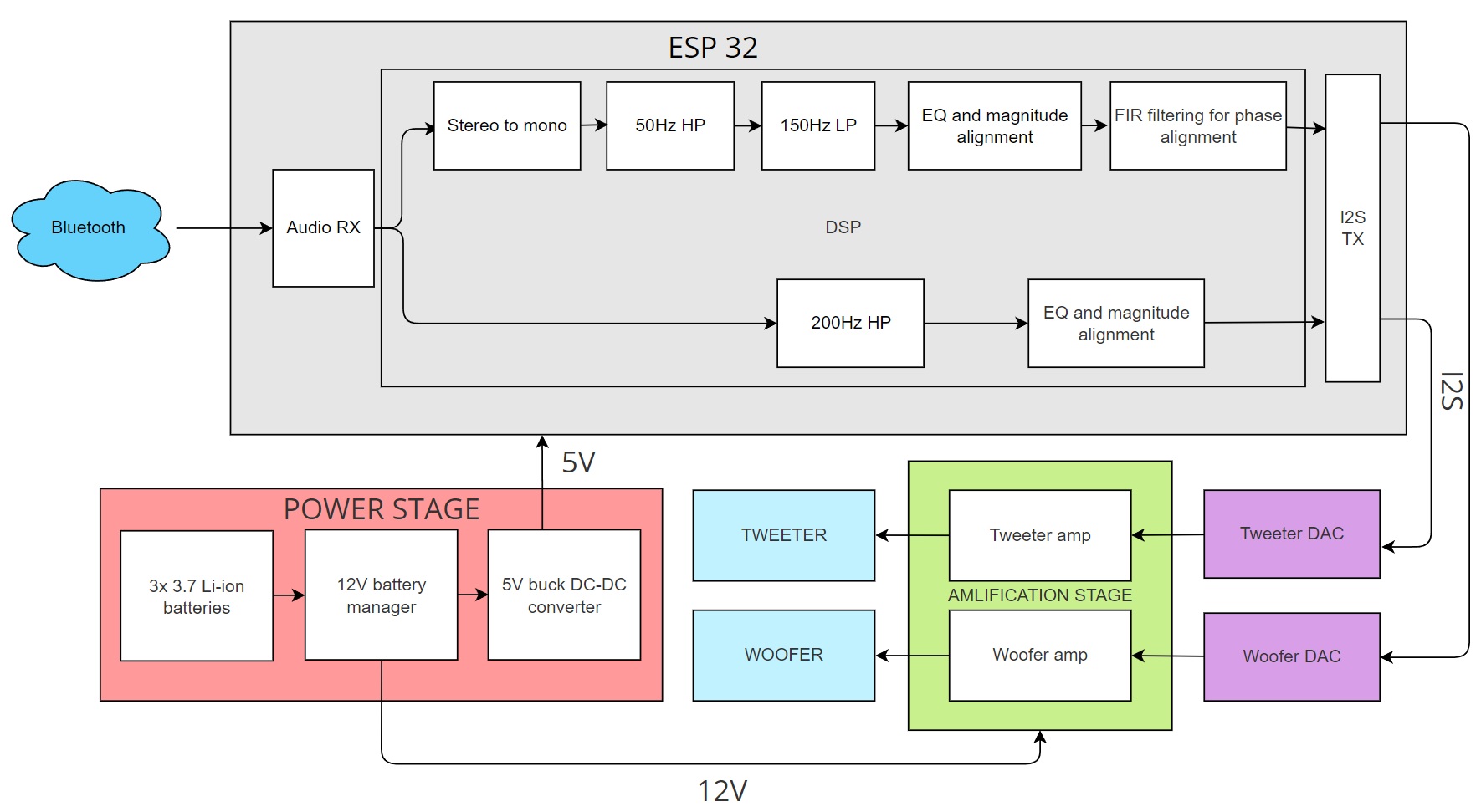
Some of the values shown on the block diagram are orientative. It will be necessary to measure the FR to determine the signal processing requiered.

Materials

Hardware

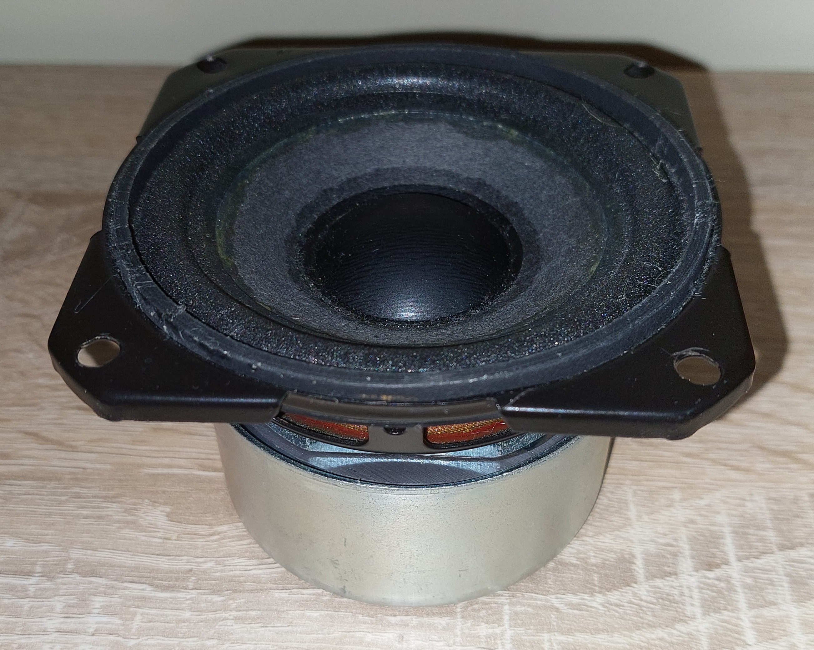
Mid-high tweeters

The drivers used for high and mid frequency stereo signal reproduction will be a pair of 2" paper cone drivers with a rated power of 5W each.

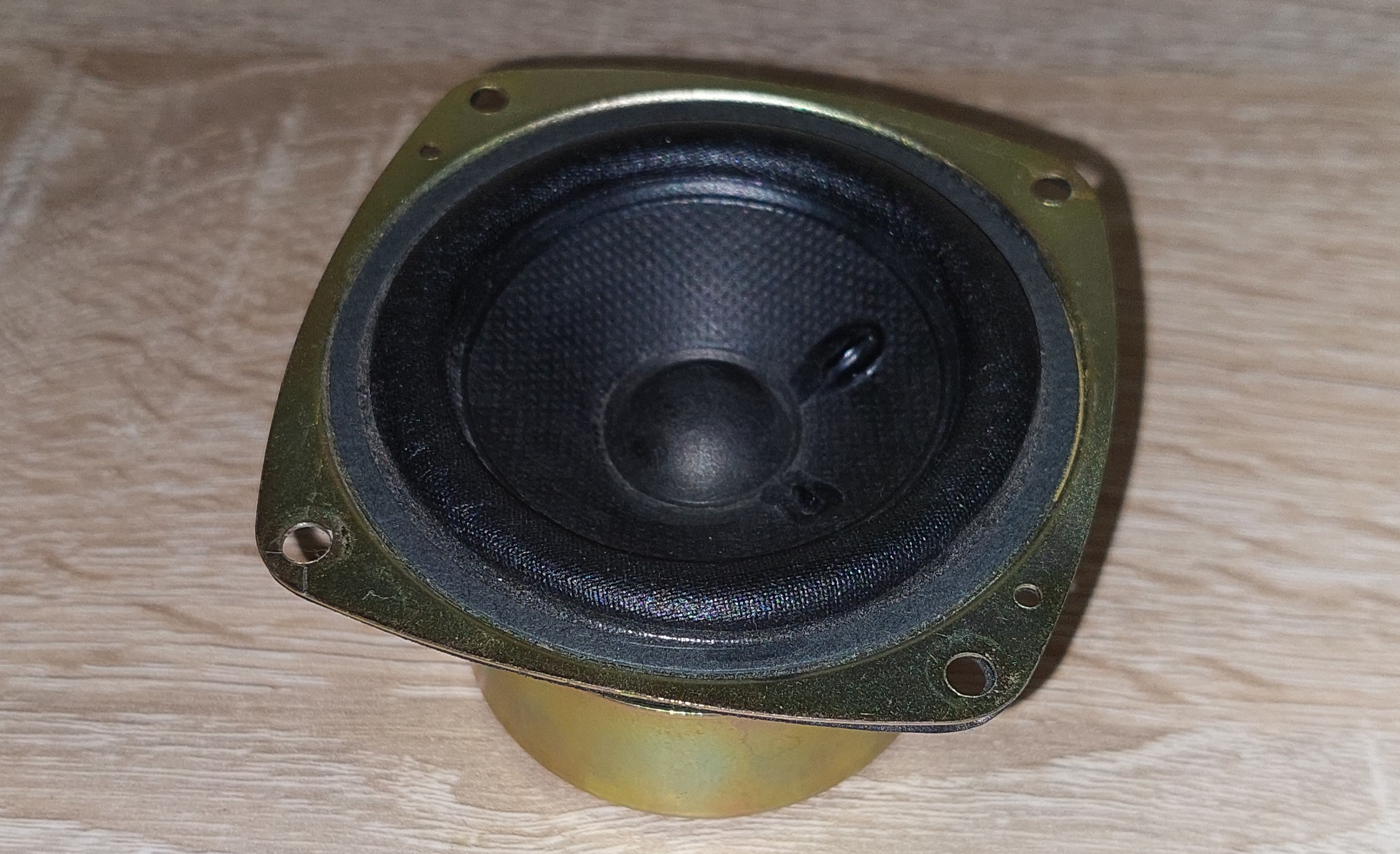
Woofer

The driver used for low frequencies mono reproduction will be a 4" paper cone driver with a rated power of 25W and very high efficency.

Microcontroller

In order to archieve the best FR the audio signal will be processed using DSP algorithms that will be coded into the µC.

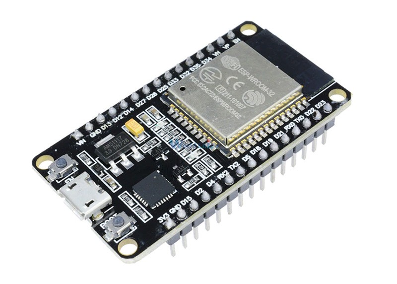
It has been decided to use the SoC ESP32 from the company Espressif for this project, because of its small size, low power consumption, low price and the fact that it has bluetooth, Wi-Fi and radio integrated.

Taking advantage of the fact that we have a µC unit, the final product could be upgraded in the future to include useful functions as power saving mode, extra bass mode, battery indicator or volume control.

DAC module

It will be needed to have 3 independent output channels. Therefore, It won’t be enough with a single stereo Digital-analog converter (DAC) unit.

By using 2 stereo DAC the system will be provided with 4 independent audio outputs.

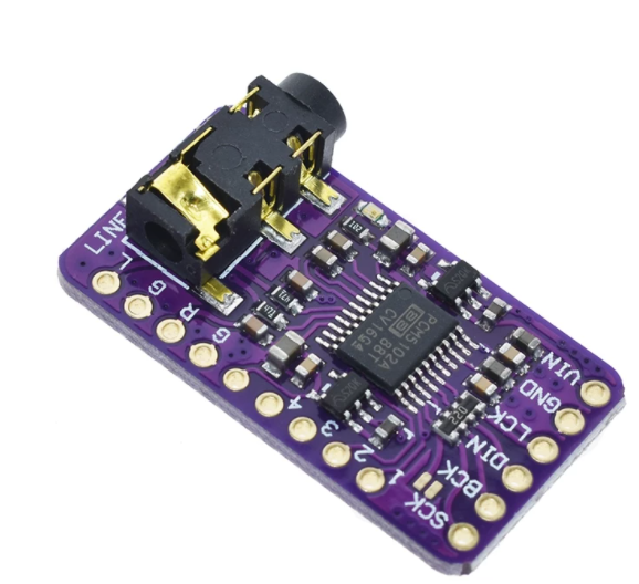
The DAC module is based on the integrated circuit (IC) PCM5102A from Texas Instruments, which is designed to work with PCM data and Inter-IC Sound (I2S) communication.

These are the fetures given by the manufacturer:

• DAC channels: 2
• DAC SRN: 112 dB
• Sampling frequency: 384 kHz
• Interface: I2S
• Data format: PCM
• Resolution: 32 bits
• Very low noise level
• Integrated high-performance audio PLL
• Intelligent mute system
• Power supply: 3.3 V or 5 V

Power amplifiers

The two tweeter drivers will be amplified by a stereo amp. On the other hand, the woofer driver will be powered with a mono amp. The amplification stage will be done with linear response amplifiers, because the audio will be received by the SoC via bluetooth in order to process it digitally, so it’s not needed to get an amplifier which includes analog filtering, for example.

The operating voltage will be 12V and, in this case, efficiency is a priority, which leds to the decision of using class-D amplifiers to improve battery life and reduce the size of the speaker.

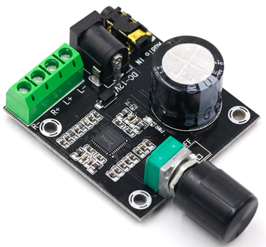
Tweeters

This is a class-D 15+15W amplifier that integrates the PAM8610 circuit, a very high quality and high efficiency amplifier that I already used time ago. In some cases, a class-D amplifier can reduce the sound quality of high frequency speakers, because it discretizes the signal in the amplification process. However, this model has a fast sampling frequency and provides a very good output signal.

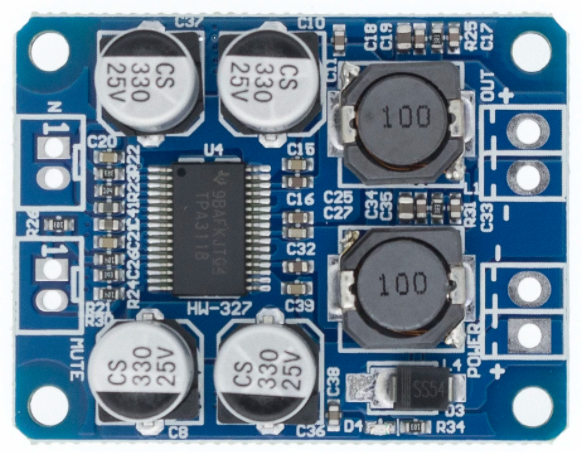
woofer

The woofer amplifier circuit uses the IC TPA3118 class-D 60W mono amplifier, which will give enough power for the woofer unit.

Battery pack

A battery pack will be built to suit the project’s power needs. It will be made out of a Battery management system (BMS) and 3.7 Li-Ion cells that provide 12V with enough current to power all the electronics at full volume.

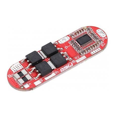
The BMS unit is based on the IC bm3451, which controls the charge and discharge cycles of a set of 3 to 5 3.7V batteries in series. By using the 3S configuration, the battery pack will deliver a nominal and maximum voltage of 11.1 V and 12.6 V, respectively.

Test equipment

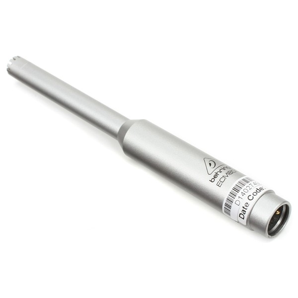
Measurement microphone

For acoustic measurements, the chosen microphone was the Behringer emc8000, which provides an omnidirectional polar pattern and a flat FR.

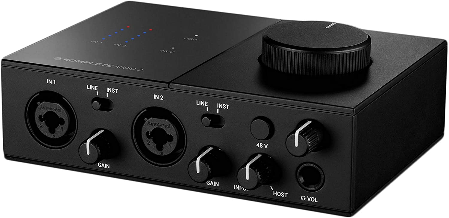
Data acquisition interface

The acoustic and electronic FR measurements were done using the sound interface Komplete Audio 2 from the company Native Instruments. This device is essentialy an ADC with its corresponding signal conditioning hardware for high precision and low noise measurements.

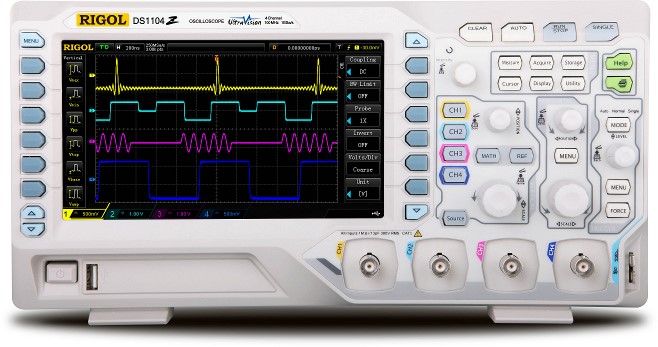
Oscilloscope

The Rigol DS1054Z oscilloscope was used to measure signal quality and channel delay and synchronization

Software

ESP-IDF

For the programming of the Espressif µC, the actual company offers a C programming environment based on the real-time operative system FREERTOS, Python scripts and CMake compiler. It also contains all the libraries and example projects needed for most of the cases.

Visual Studio Code

The IDE chosen was VS Code, an open-source code editor and programming environment released by Microsoft. From this software, it is possible to open a terminal and call commands to build and flash the code into the µC.

MatLab

Matlab will be used for filter design purposes and TF simulation, which includes the discretization process of continuous filters.

WinISD

WinISD is a simulation software which eases the task of designing speaker enclosures given the desired design parameters and electro-mechanical coefficients of a physical driver.

Room Equalizer Wizard

Room Equalizer Wizard is an open-source software meant to do room acoustics measurements. Which is interesant about this software is that it can be used to measure frequency responses of electric signals, plotting a very accurate bode diagram of the system. Then, it will be used for acoustic measurement of the drivers, as well as the DAC output FR. Another useful feature of this software is the frequency-dependant impedance measurements and Thielle-Small parameter calculation, which will be used to measure the modelling variables required by WinISD in order to design the speaker enclosure.

Fusion360

This software will be used to design the enclosure of the speaker, as well as preparing the files required for the 3D printer and the laser CNC cutter.

Design process

Enclosure design

The earlier project stages have the biggest impact on the final result. Therefore, to achieve a flat FR, it is necessary to start with a good-sounding enclosure.

Driver’s free-air frequency response measurement

To make a decision about the enclosure dimensions and frequency tuning, it is convenient to do an open-baffle measurement of the driver[1]. The testing equipment includes a mount for the drivers, a measurement microphone and a sound interface with +48V phantom power.

The resulting FR can give a brief idea of what can be expected of the final FR. The results are the following.

Woofer

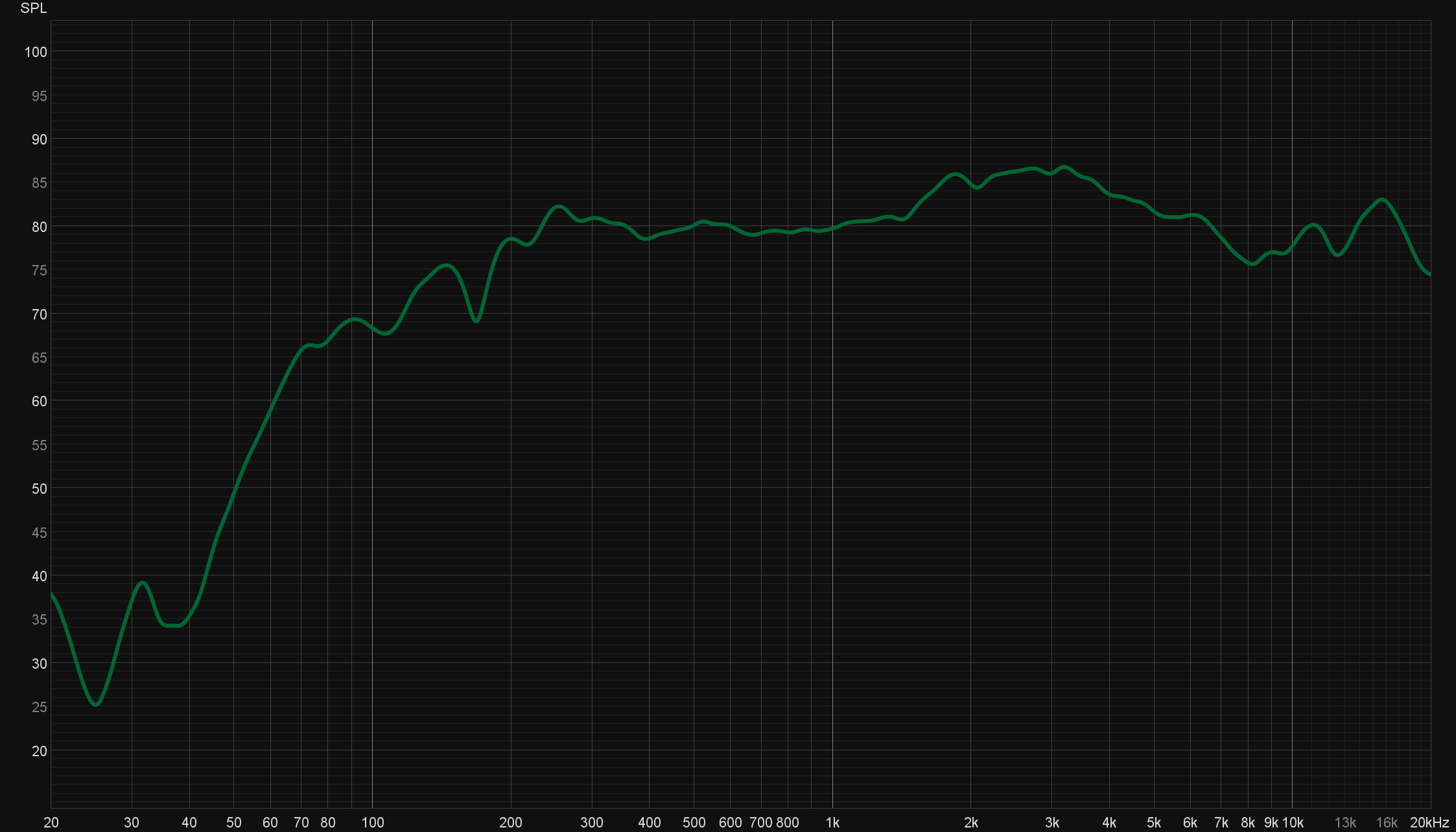
As shown in the following bode diagram, the woofer driver will reach 90Hz with ease. By using a bass reflex enclosure and DSP bass enhancements we can expect it to reach the 75Hz mark.

Tweeter

On the other hand, the tweeter driver has a better response in the high-frequency section, whereas the sound pressure in the bass section is reduced. By looking at the bode diagram, the tweeter enclosure and the crossover frequency should be tuned to match a cutoff frequency of 200Hz.

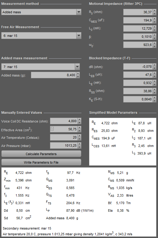
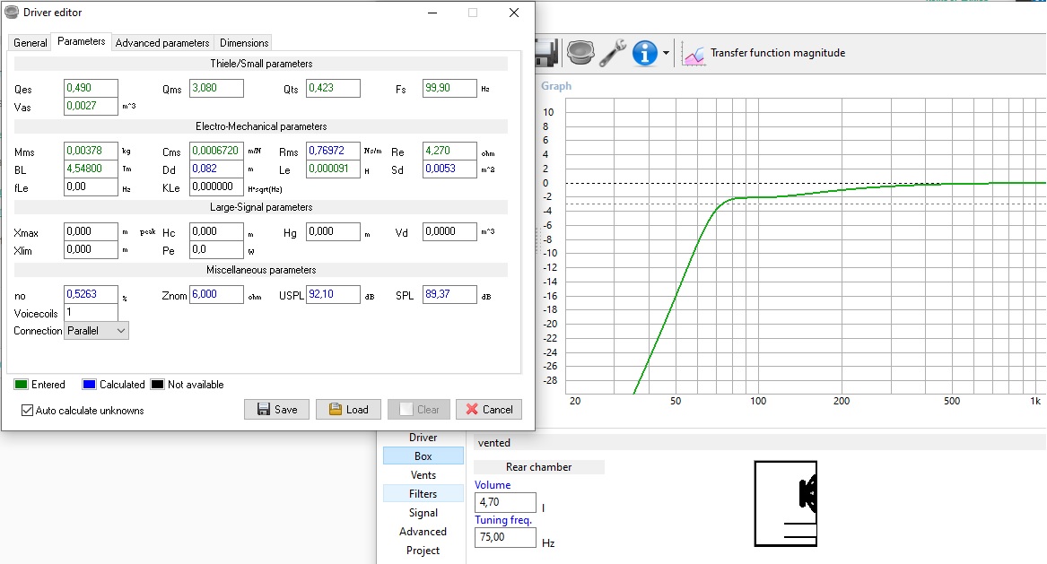
Driver’s electro-mechanical coefficients measurement

To begin with the enclosure design it is needed to measure the Thielle-Small parameters [2] of the drivers.

These parameters are a set of electro mechanical modelling parameters that measure the driver’s behaviour at low frequencies. They can be used to simulate the FR of speaker baffles for a certain driver. The software REW will be used for that purpose.

REW uses a model for the electrical impedance component of the driver based on “Electrodynamic Transducer Model Incorporating Semi-Inductance and Means for Shorting AC Magnetization”[3].

The mechanical impedance model incorporates elements that cater for the frequency-dependence of compliance. It uses the LOG model of viscoelasticity, from “Low-Frequency Loudspeaker Models That Include Suspension Creep” [4].

This model calculates the electro-mechanical coefficients of a driver from its impedance data. By using REW, the impedance can be measured and then use the obtained data to calculate the modelling parameters.

The needed equipment includes an audio interface with two or more input channels and a measuring probe that can be built by following the next electric diagram.

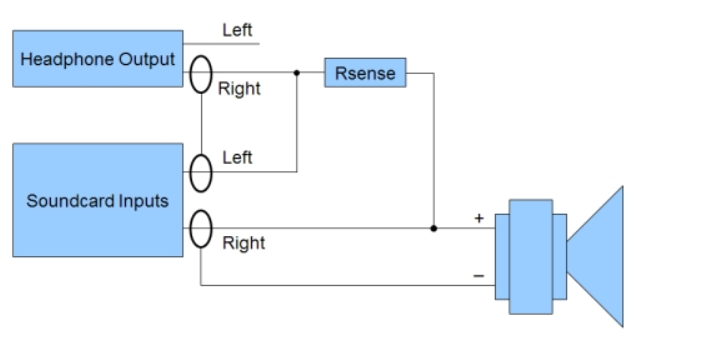
It is important to calibrate the probe previously, which includes measuring the impedance of the terminals and the audio output of the interface.

There are several methods that we can use for measuring the thielle-small parameters of a loudspeaker. In this case, we are going to use the added mass method, due to its simplicity and accuracy.

This methods requires to measure the impedance of the driver in 2 different conditions.

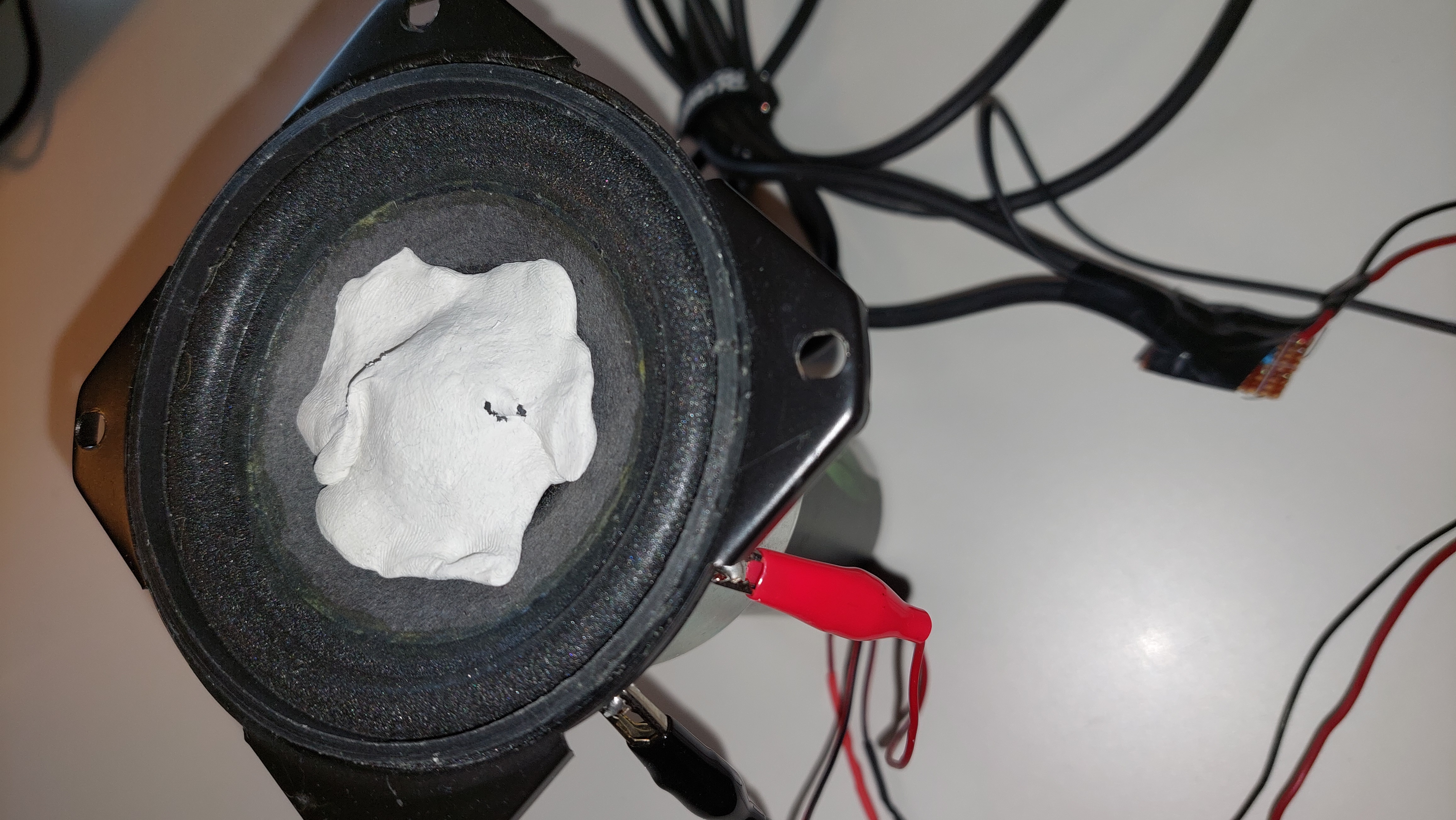
Scenario 1: Free-air impedance measurement

The first one is the free-air measurement, which consists of measuring the driver horizontally, letting the cone vibrate freely in the air.

Scenario 2: Added-mass impedance measurement

Impedance measurements results

Note

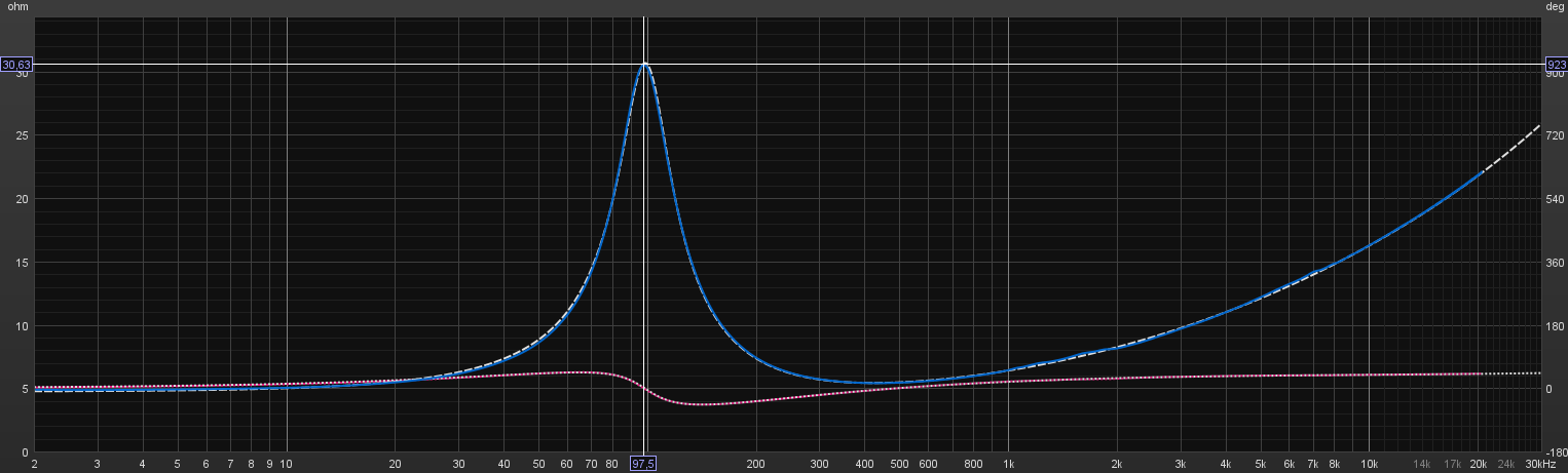
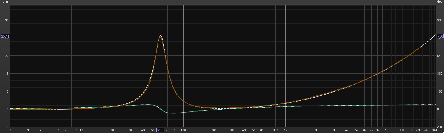
The impedance peak that we see represents the resonant frequency of the driver. As we can see, its magnitude and frequency are reduced when we add some mass to the cone. The reason for this is that the mechanical model of a loudspeaker is essentially a suspended mass system with added complexity caused by other physical properties as, for example, the air compilance.

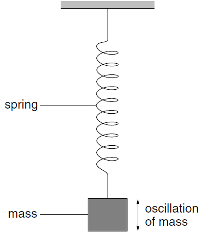
In a suspended mass oscillator, the heavier the mass, the lower the resonant frequency.

With the measurements that were done, REW can calculate the Thielle-Small parameters.

Enclosure simulation

After measuring both the tweeter and the woofer parameters, they can be introduced into the simulation software. This will be done by using WinISD.

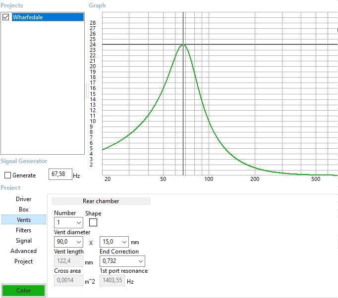
The woofer baffle will be a bass-reflex enclosure[1]. This type of design is based on a second order system which includes a resonance at the tuning frequency, and gives a steeper rollof on the lower frequencies. In other words, it Increases the magnitude at the tuning frequency by reducing the energy output at frequencies below.

As one of the objectives is achieving a high-efficency speaker with a long battery life, increasing the BW to cover those frequencies that can be reproduced easily while attenuating the ones that are more power-hungry is a wise decision.

After introducing the parameters into the driver properties, the tuning frequency and volume of the enclosure can be adjusted. It is intended to extend the bass response as possible, but as a counterpart, if the resonant frequency is set too low, it will create a dip in the magnitude of the frequencies above the tuning frequency.

Based on the two conditions mentioned above, the tuning frequency was adjusted to 75Hz, which is the sweet spot where the BW is extended the most without compromising the higher bass frequencies excessively.

About the volume, as it increases, the bass port resonance and the frequencies above increase as well in terms of magnitude. It was finally adjusted to 4,7 liters, which is a reasonable size that won’t result on an excessively big enclosure and doesn’t make the port resonance too pronounced.

Once these two parameters were defined in the software, the bass port area has to be defined so the software can calculate the tube length.

As the surface area is increased, the port air velocity is reduced. A high air velocity introduces resonances in the final FR, causing harmonic distortion. This is something to take into consideration, as distortion is desired to be as low as possible. The limitation is that, as the surface is increased, the tube has to be larger in order to resonate at the desired frequency.

To decide the port area, taking into account the conditions above, the input power was set to 20W, which is slightly above the maximum power that is going to be applied to the woofer. Then, the air velocity inside the port can be plotted for that output power.

As documented in many speaker enclosure design guides, it should not exceed the 25 m/s mark at the resonant frequency, because at this point, the port distortion starts to be audible and it increases exponentially

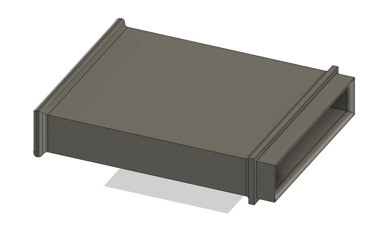
Enclosure 3D modelling

After the enclosure volume and tube shape has been determined, the continuing process lies in the enclosure modelling.

Once a design was decided to be the best one among some other sketches in terms of appearence, strucure consistency, practicity and simplicity, the enclosure was modeled to match the calculated parameters.

The first step was to measure the driver’s dimensions. With those dimensions, some sketches were drown on Fusion 360, and then, they were extruded to create the parts of the enclosure.

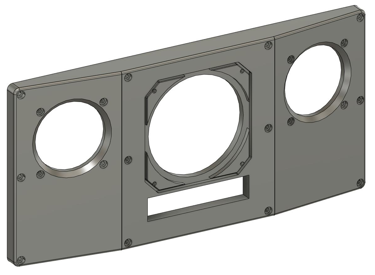
The image below shows an example of the modelling process.

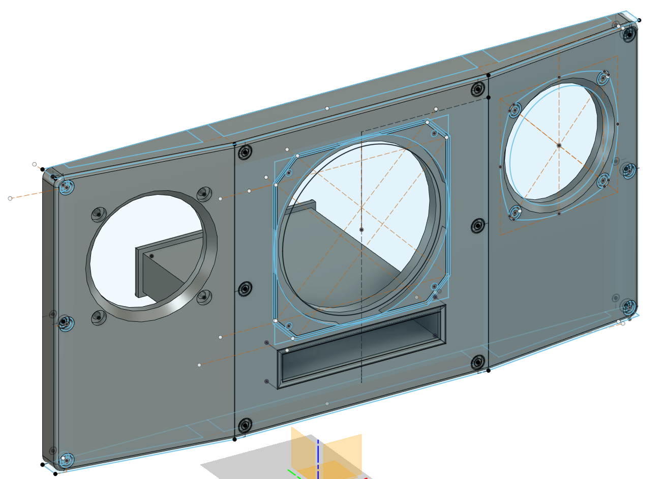
Considering that the front of the enclosure is going to be 3D-printed, it is convenient to separate some parts like the tube, because if something bad happens during the printing process, or the calculations were mistaken, it won’t be necessary to discard the entire part.

The tube is specially susceptible of miscalculations. Even a length offset of a few millimeters can change the resonant frequency of the tube, thus changing the bass response. Therefore, even considering that it would have been easy to print the front panel and the tube together, it was better to separate it.

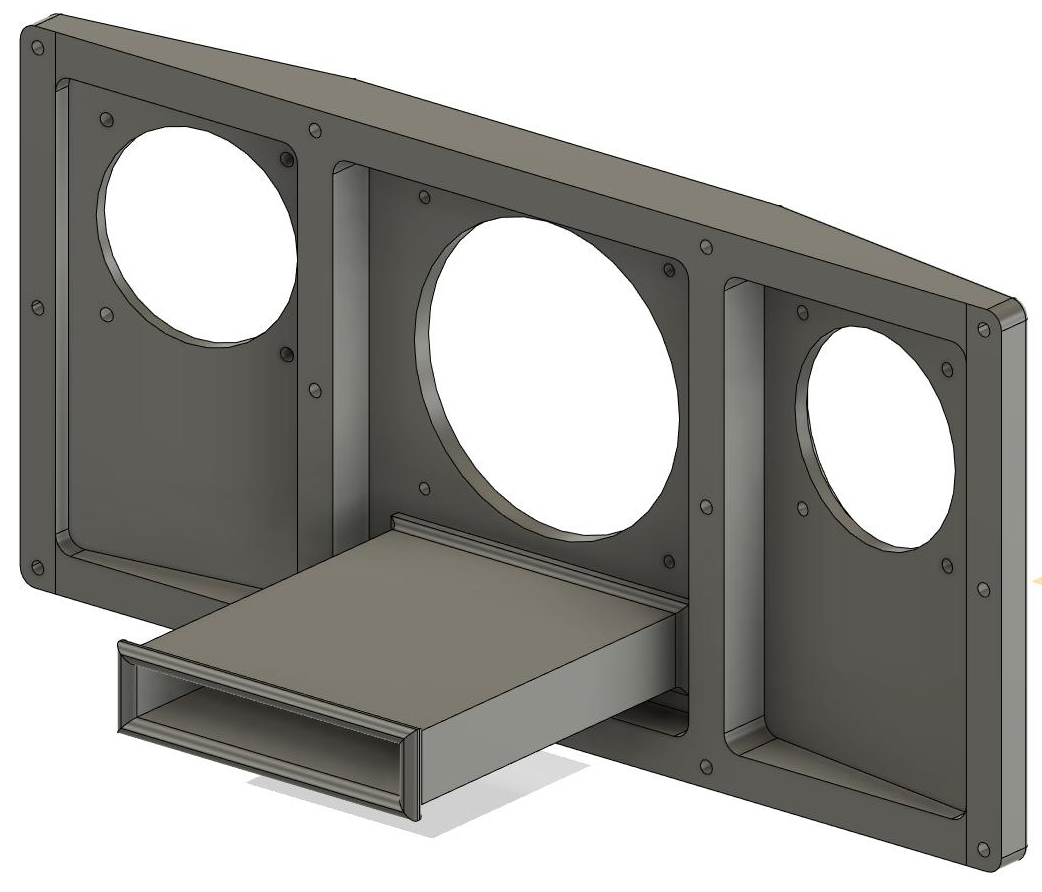
Metallic treads were added for the screws, which makes the product much more durable if it’s going to be assembled and disassembled regularly, which was expected to be a future task of the project. For that purpose, insertions were added in order to put nuts inside the screw holes. Finally, an exploded view of the full enclosure.

Finally, an exploded view of the full enclosure.

Considering the frequency range that the speaker is going to reproduce, some research was made to decide the width of the enclosure walls. It was chosen to be 12 mm wide, printed with a 50% infill. The sound will be good enough and the speaker won’t be too heavy.

Implementation

These are the steps taken in the implementation process. The earlier steps need to be completed in order to continue with the later ones.

1. Digital stage assembly
2. Digital data receiver programming (bluetooth)
3. DSP algorithm developing
4. Full system implementation
5. Filter adjustement and FR correction

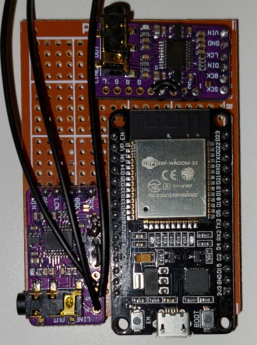
Digital stage assembly

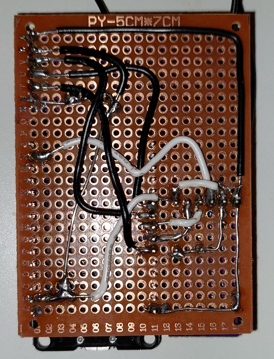
The digital stage is composed by the two DAC circuits and the µC. Audio will be received by the µC as bluetooth data, convert it into PCM format and transfer it to the DAC by using the I2S peripheral. The two DAC modules were assembled in a prototype PCB connected to the µC.

Digital bluetooth data receiving programming

At this point, the next thing to do is programming and testing the ESP32 to ensure that the data is being received and transmitted correctly. To start with it, it is needed to download the ESP-IDF tools for Espressif devices. It can be found in the official website of the manufacturer [5]. This pack includes example projects for various applications. Each one already incorporates the FREERTOS libraries and the C structures needed to configure operation modes and peripherals. One of these projects is a2dp_sink, which is basically a bluetooth audio receiver that incorporates I2S communication with PCM DACs. By building and flashing the project onto the µC, it was noted that some things needed to be changed:

• The output volume of the signal couldn’t be changed.
• Every 10 seconds the output volume raised by a 10% automatically
• The program is configured for 2.0 stereo and it needs to be 2.1

The first problem mentioned was caused by the fact that the code did not include a function to multiply each audio sample with the gain desired, even though there is a 7-bit variable that stores the volume value numerically.

The variable data allocates the sample value in the memory of the ESP32 using PCM format, those samples being written by the ring-buffer that receives them via bluetooth. The function assigned for this task is called I2S_Task_Handler, and it is also responsible of sending data blocks through the I2S interface.

Knowing that, it’s easy to implement the desired function.

bt_i2s_task_handler function in bt_app_core.c:

102
103
104
105
106
107
108
109
110
111
112
113
114
115
116
117
118
119
120
121
122
123
124
125
126
127
128
129
130
131
132
133
134
135
136
137
138
139
140
141
142
143
144
145
146
147
148
149
150
151
152
153
154
155
156
157

static void bt_i2s_task_handler(void *arg)
{
    uint8_t *data = NULL;
    size_t item_size = 0;
    size_t bytes_written = 0;


/* RECEIVE DATA FROM RINGBUFFER AND WRITE IT TO I2S DMA TRANSMIT BUFFER */
    for (;;) {
     data = (uint8_t *)xRingbufferReceive(s_ringbuf_i2s, &item_size, (TickType_t)portMAX_DELAY);
        if (item_size != 0)
        {
			int16_t * pcmdata = (int16_t *)data;
			for (int i=0; i<item_size/2; i++) {
				int16_t temp = *pcmdata;
				temp = temp * logarithm[volume_step];
				*pcmdata = (int16_t)temp;
				pcmdata++;
		}

			// NEW POINTER FOR PARALLEL PROCESSING
            uint8_t* backup = (uint8_t*) malloc(item_size);

            // COPY SAMPLES FROM DATA TO BACKUP
            for (int i=0; i<item_size; i++)
            {
              	*backup = *data;
            	data++;
            	backup++;
            }

            // SET POINTERS BACK TO THEIR ORIGINAL POSITION
            for (int c=0; c<item_size; c++)
            {
            	data--;
            	backup--;
            }

            // SIGNNAL PROCESSING
	 		process_woofer(data, item_size);
			process_tweeter(backup, item_size);


	        // DAC0 AND DAC1 WRITE
			i2s_write(0, data, item_size, &bytes_written, portMAX_DELAY);
			i2s_write(1, backup, item_size, &bytes_written, portMAX_DELAY);


            vRingbufferReturnItem(s_ringbuf_i2s,(void *)data);

            // RELEASE DYNAMIC MEMORY USED BY BACKUP
            free(backup);
        }
    }
}

The logarithm variable is a lookup table that represents a discretization of a log10 function in 16 steps in total, and is a more efficient alternative than using the <math.h> library functions. This is neccesary to control the volume consistently, because the human psychoacoustic perception of sound pressure works in a logarithmic scale [6].

Then, a criteria is established for dB increments in volume. 100% means 0dB, and from there, a constant amount of decibels is subtracted each step, in this case, being -2 dB. Therefore, the first step is -inf dB, the second one -30 dB, the third one -28 dB and this series continues until the last step, 0dB, which is the same as a 1 in the linear scale.

After this, we have to convert our dB steps into linear scale gain, which is the one that will be multiplied by the samples in order to achieve the desired output.

This conversion can be made with this equation: $$Gain = 10^\frac{dB}{20}$$

By using this formula, the next lookup table is created.

The implementation in the code is as follows.

discretization of log10 function in in bt_app_core.c

12
13

extern uint8_t s_volume;
static uint8_t logarithm[16] = {0, 0.03, 0.05, 0.06, 0.08, 0.1, 0.13, 0.16, 0.2, 0.25, 0.32, 0.4, 0.5, 0.63, 0.79, 1};

The last thing to do to stream audio in 2.1 format is configuring the second i2s peripheral with the same parameters as the first one.

i2s channel and pinout configuration in main.c:

166
167
168
169
170
171
172
173
174
175
176
177
178
179
180
181
182
183
184
185
186
187
188
189
190
191
192
193
194
195
196
197
198
199
200
201
202
203
204
205
206
207
208
209
210
211
212
213

 /* I2S configuration parameters for channel 1*/
    i2s_config_t i2s_config = {
        .mode = I2S_MODE_MASTER | I2S_MODE_TX,              /* only TX */
        .sample_rate = 44100,
        .bits_per_sample = 16,
        .channel_format = I2S_CHANNEL_FMT_RIGHT_LEFT,       /* 2-channels */
        .communication_format = I2S_COMM_FORMAT_STAND_MSB,
        .dma_buf_count = 16,
        .dma_buf_len = 128,
        .intr_alloc_flags = 0,                              /* default interrupt priority */
        .tx_desc_auto_clear = true                          /* auto clear tx descriptor on underflow */
    };

    /* enable I2S channel 1*/
    i2s_driver_install(0, &i2s_config, 0, NULL);

    i2s_pin_config_t pin_config = {
        .bck_io_num = 27,
        .ws_io_num = 33,
        .data_out_num = 32,
        .data_in_num = -1                                   /* not used */
    };
    i2s_set_pin(0, &pin_config);

    /* I2S configuration parameters for channel 2*/
    i2s_config_t i2s_config_2 = {
        .mode = I2S_MODE_MASTER | I2S_MODE_TX,
        .sample_rate = 44100,
        .bits_per_sample = 16,
        .channel_format = I2S_CHANNEL_FMT_RIGHT_LEFT,
        .communication_format = I2S_COMM_FORMAT_I2S_MSB,
        .dma_buf_count = 16,
        .dma_buf_len = 128,
        .intr_alloc_flags = 0,                              /* default interrupt priority */
        .tx_desc_auto_clear = true                          /* auto clear tx descriptor on underflow */  
};

    /* enable I2S channel 2*/
    i2s_driver_install(1, &i2s_config_2, 0, NULL);
    
    i2s_pin_config_t pin_config_2 = {
        .bck_io_num = CONFIG_EXAMPLE_I2S_BCK_PIN,
        .ws_io_num = CONFIG_EXAMPLE_I2S_LRCK_PIN,
        .data_out_num = CONFIG_EXAMPLE_I2S_DATA_PIN,
        .data_in_num = -1                                                     
    };

    i2s_set_pin(1, &pin_config_2);

The value assigned to the variable .dma_buf_len was changed from 64 to 128, because as it is needed to double the amount of data transmitted than when it was configured for using only one DAC, the ringbuffer also needs to be two times bigger. Omitting to do so will result in playback problems as missing samples and noises.

DSP algorithm implementation

Once the audio samples are registered into the μC, they will split into the two paths that were exposed in the block diagram at the beginning of the document. Therefore, two functions will process these samples. One will process the woofer channel and the other will work with the stereo tweeter channel.

Woofer processing introduction

• The first thing to do is obtaining a 2.1 signal, which means that one of the two stereo signals needs to be converted into mono. This is done by using a monosum algorithm, which sums the right and left sample into the output sample. At this point, only one signal is being processed.
  Note

  Note that samples are being stored on a 32-bit variable. This is mandatory because when doing a monosum, the amplitude of both samples is being joined, resulting into a greater magnitude final sample.
• The next proceess consists on adding the low-pass filter needed to make the crossover. At this moment, the gain is adjusted to avoid overflow in the next process.
• The third process is a peaking filter that is used to correct the FR after acoustic measurements were made (will be explained in more depth below).
• The fourth process is a limiter which saturates the signal if it surpasses the overflow limit.
• The last process consists on muting one of the two DAC's channels and sending the processed sample to the other channel.

This is the resulting function.

Woofer processing function in dsp.h

 1
 2
 3
 4
 5
 6
 7
 8
 9
10
11
12
13
14
15
16
17
18
19
20
21
22
23
24
25
26
27
28
29
30
31
32
33
34

static void process_woofer (uint8_t * data, size_t item_size) {

	int16_t *samples = (int16_t *) data;
	int16_t *outsamples = (int16_t *) data;


	for (int i=0; i<item_size; i=i+4)

	{
		//COPY SAMPLES AND MAKE MONOSUM
		int32_t preinsample =  *samples;
	    samples++;
		preinsample +=  *samples;
	    samples++;
	    float insample = (float) preinsample;
	    
	    // LOW PASS FILTER
	    insample = lpf_200Hz_W_ZOH(insample)*0.25;  //GAIN ADJUSEMENT
	    
	    // 78Hz BOOST
	    insample = Wf_78Hz_Boost(insample);

        // OVERFLOW PROTECTION
	    if(insample >= 16383){insample = 16383;}
	    else if(insample <= -16383){insample = -16383;}

	    //SEND MONO SAMPLE INTO ONE OUTPUT CHANNEL
		*outsamples = 0; //MUTE THE LEFT CHANNEL
		outsamples++;
	    *outsamples = ((int16_t) insample); //SEND TO RIGHT CHANNEL
		outsamples++;

	}
}

Tweeter processing introduction

• The first process is the high-pass filter that, in combination with the low-pass filter applied to the woofer channel, make up the crossover.
• Then, after the acoustic FR is measured, it is corrected with peaking (bell) filters.
• Lastly, both left and right samples are sent to the DAC on PCM format.

This is the resulting function.

 1
 2
 3
 4
 5
 6
 7
 8
 9
10
11
12
13
14
15
16
17
18
19
20
21
22
23
24
25
26
27
28
29
30

static void process_tweeter (uint8_t * data, size_t item_size) {

	int16_t * samples = (int16_t *) data;
	int16_t * outsamples = (int16_t *) data;


	for (int i=0; i<item_size; i=i+4)
	{
		//COPY EACH SAMPLE IN A DIFFERENT VARIABLE
		float insampleL = (float) *samples;
	    samples++;
		float insampleR = (float) *samples;
		samples++;

		// PROCESS SAMPLES WITH 200 Hz High-pass
		insampleL = hpf_200Hz_L(insampleL);
		insampleR = hpf_200Hz_R(insampleR);


		// PROCESS SAMPLES WITH 2KHz Bell Cut
		insampleL = Wf_2kHz_Cut_L(insampleL);
		insampleR = Wf_2kHz_Cut_R(insampleR);

		*outsamples = (int16_t) insampleL;
		outsamples++;
		*outsamples = (int16_t) insampleR;
		outsamples++;
	}

}

Now that a brief introduction to the signal processing functions has been given, a deeper look into the individual processes will be taken.

Crossover design and discretization method comparison

To prevent phase issues, It is mandatory to have the same phase response in the cutoff frequency [7].

As the tweeter enclosure is sealed, There is already a first order system which has a +90 degree phase shift in its rollof. It is intended to create a second order crossover, which means that the tweeter channel will implement a first order high pass, while the woofer low pass filter will be a second order one in order to match the +180 phase. Both cutoff frequencies must be equal.

IIR design can be done in the continuous domain, and then, discretize it. The most common discretization method for this purpose is Tustin. Different discretization methods will be evaluated by measuring the signal quality out of the DAC.

Woofer low pass IIR filter

The next task will be adding the LPF seen in the code, which is the one that sets the crossover at 200Hz.

The most efficient way to create a second order TF with a cutoff frequency and damping factor that we desire is to use a normalized polynomial for butterworth filters.

The denominator of a second order butterworth filter with a Wn of 1 rad/s is defined by this expression:

$$(s^2+1.414214s+1)$$

Now it is known that the damping factor (ζ) must be 1.414214, which results in a quality factor of 0.707.

By knowing that the cutoff frequency is going to be 200 Hz -> 1250 rad/s, the filter’s TF can be designed as follows.

The filter TF must be: $$\frac{1250^2}{s^2+1.414 \cdot 1250s+1250^2}$$

After discretizing the filter using ZOH method, the next discrete TF is obtained:

$$\frac{0.0003964 z + 0.0003911}{z^2 - 1.96 z + 0.9607}$$

The resulting difference equation is:

$$Y_{k} = U + 0.0003964U_{k-1} + 0.0003911U_{k-2} + 1.96Y_{k-1} - 0.9607Y_{k-2}$$

This equation can be implemented in the code as a function.

Low-pass butterworth filter algorithm in dsp.h

 1
 2
 3
 4
 5
 6
 7
 8
 9
10
11
12
13
14
15
16
17

static float wy = 0;
static float wy_1 = 0;
static float wy_2 = 0;
static float wu_1 = 0;
static float wu_2 = 0;

static float lpf_200Hz_W(float wu)
{
	wy =  wu_1 * 0.0003964 + wu_2 * 0.0003911 + wy_1 * 1.96 - wy_2 * 0.9607;

	wu_2 = wu_1;
	wy_2 = wy_1;
	wy_1 = wy;
	wu_1 = wu;

	return wy;
}

Once the code is compiled and flashed into the µC, it is possible to measure the TF of the DAC output for a frequency sweep to obtain a bode diagram of the process.

On the other hand, if the TF is discretized with the Tustin method, the result is as follows:

$$\frac{0.0001969 z^2 + 0.0003937 z + 0.0001969}{z^2 - 1.96 z + 0.9607}$$

The resulting difference equation is:

$$Y = 0.0001969U_{k} + 0.0003937U_{k-1} + 0.0001969U{k-2} + 1.960Y_{k-1} - 0.9607Y_{k-2}$$

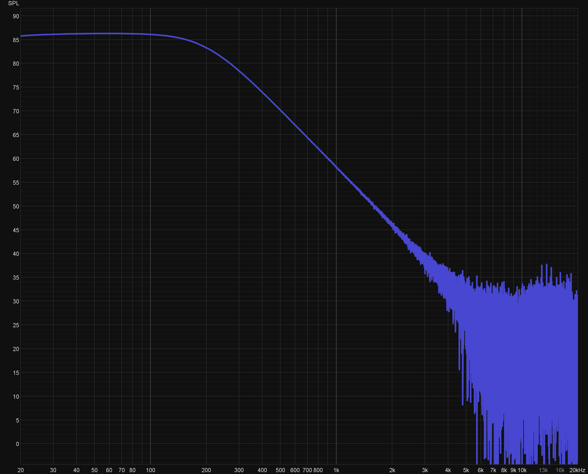
It is clear that there is no difference in terms of FR. It is also important to look at other parameters to compare how the signal quality gets compromised in each of these discretization methods.

By looking at the distortion and background noise, it can be concluded that both filters behave similarly.

Tweeter high pass IIR filter

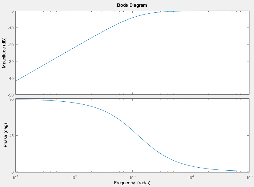
The design process for the HPF algorithm starts by creating a TF with the desired characteristics.

Due to the fact that the tweeter enclosure is sealed, instead of a 2nd order filter, it is needed to design a 1st order high-pass filter with a cutoff frequency of 200Hz, so let’s begin by constructing the TF and simulate it in matlab.

• The filter must have a +20dB/dec slope from 0Hz to 200Hz. -> Derivator
• The slope from 200Hz onwards must be 0dB/dec. -> Pole with natural frequency of 200Hz

This is the resulting TF

$$\frac{s}{s+1250}$$

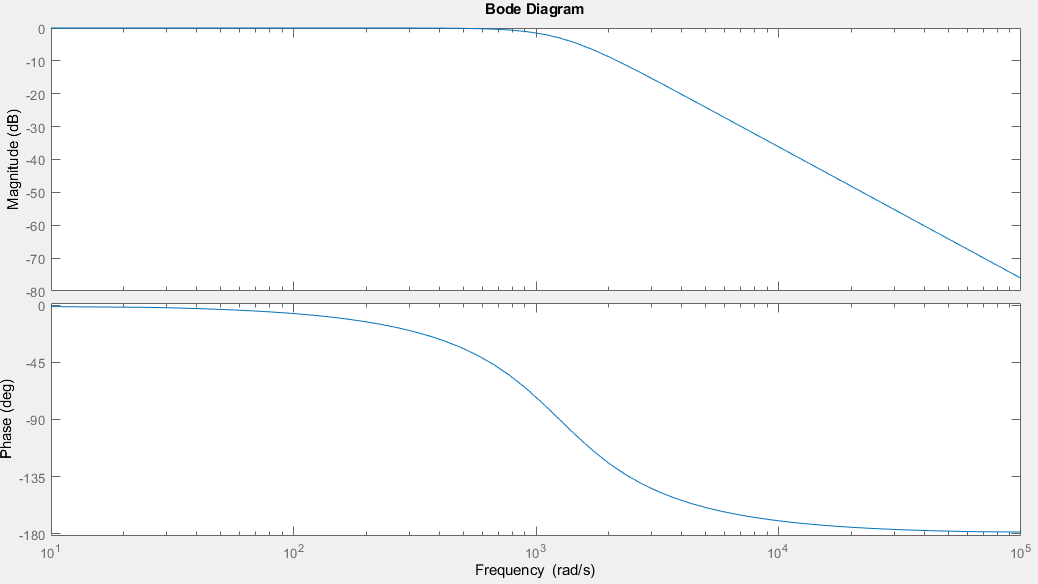
This is the the system’s response represented in a bode diagram.

Now the filter will be discretized using the ZOH method with a sampling frequency of 44.100Hz, which is the sampling frequency configured in the ESP32 code. This is the TF of the filter in the discreet domain.

This is the TF of the filter in the discreet domain:

$$\frac{z-1}{z-0.9721}$$

The resulting difference equation is as follows.

$$Y_{k}=U_{k}-U_{k-1}+0.9721Y_{k-1}$$

The implementation in C is as follows:

200 Hz High-Pass filter algorithm in dsp.h

 1
 2
 3
 4
 5
 6
 7
 8
 9
10
11
12
13
14
15
16
17
18
19
20
21
22
23
24
25

static float ly = 0;
static float ly_1 = 0;
static float lu_1 = 0;

static float ry = 0;
static float ry_1 = 0;
static float ru_1 = 0;

// LEFT CHANNEL FILTER
static float hpf_200Hz_L(float u)
{
	ly = u - lu_1 + 0.972053270286608 * ly_1;
	ly_1 = ly;
	lu_1 = u;
	return ly;
}

// RIGHT CHANNEL FILTER
static float hpf_200Hz_R(float u)
{
	ry = u - ru_1 + 0.972053270286608 * ry_1;
	ry_1 = ry;
	ru_1 = u;
	return ry;
}

After compiling the code, the DAC output FR was measured.

Full system implementation

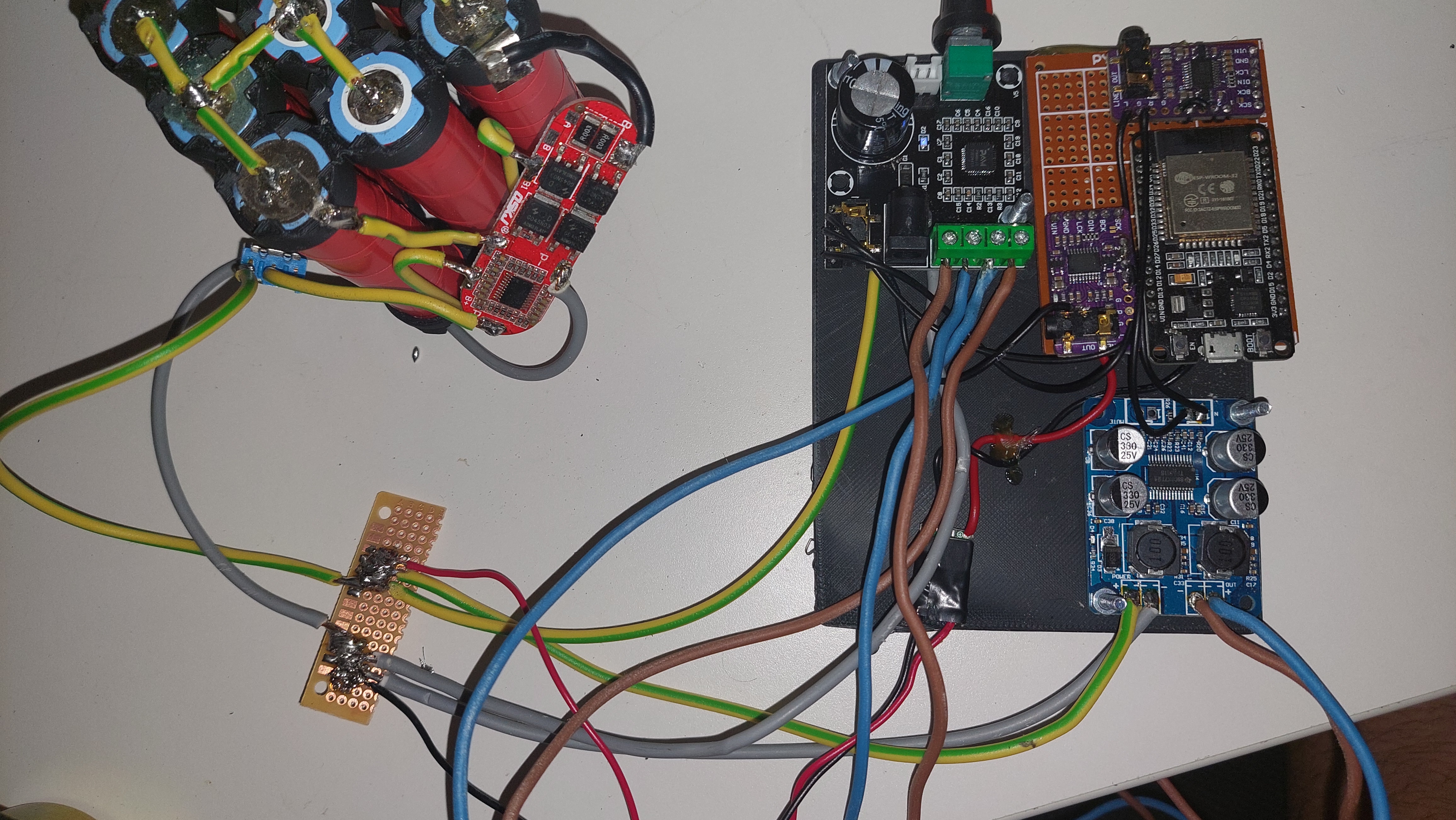
Hardware assembly

All the hardware components were connected and powered by the battery pack. To make it more robust, a 3D printed plastic plate was used to allocate each piece in its place.

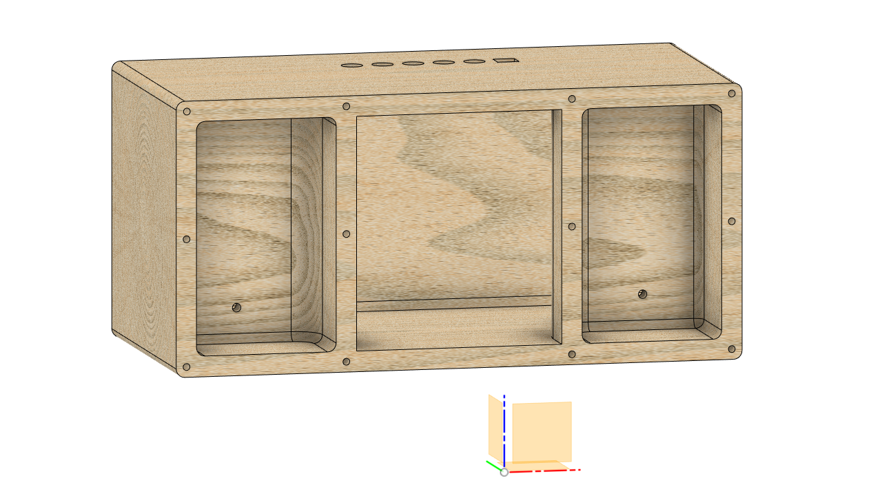
Enclosure building

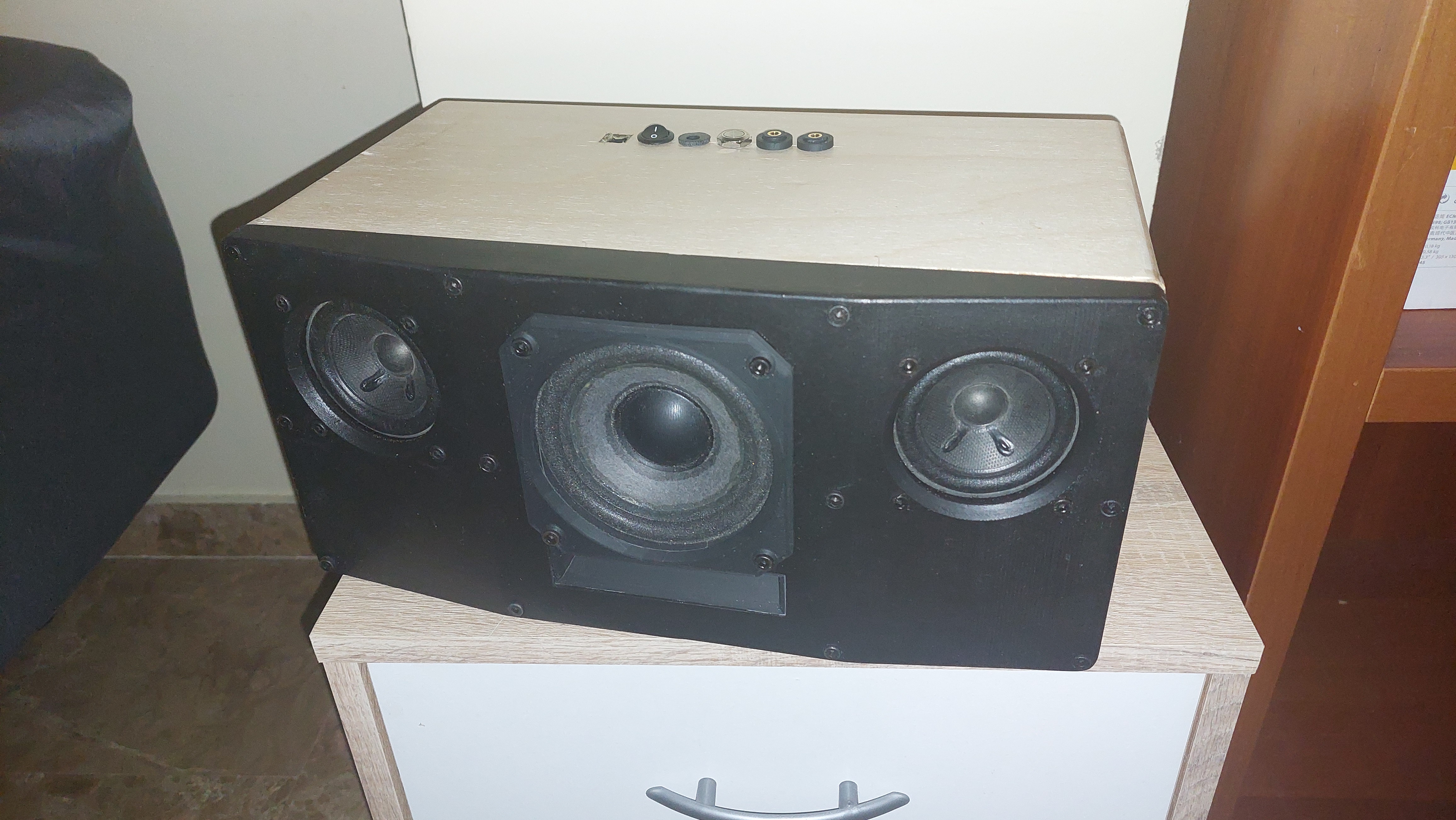
The wooden part of the enclosure is made from two layers of 6cm thick plywood that were cut by a laser cutter. After all the pieces were glued together, screw nuts were added to make it easier to open the enclosure in the future.

The wood was treated with hydrophobic varnish to prevent water and environmental damage. As a last step, a rubber seal was glued over the nuts.

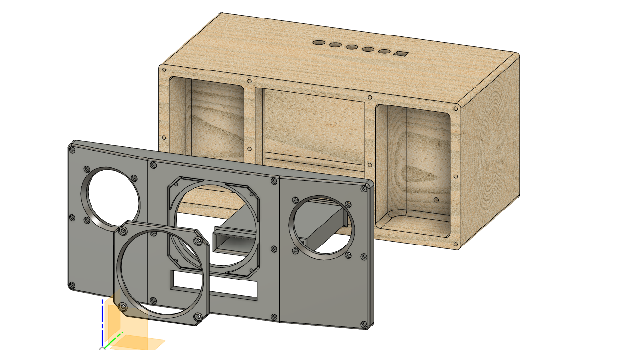
The front cover was printed using ABS plastic. After that, some sanding was needed to prepare the surface for painting. Finally, the piece was painted with acrylic spray paint.

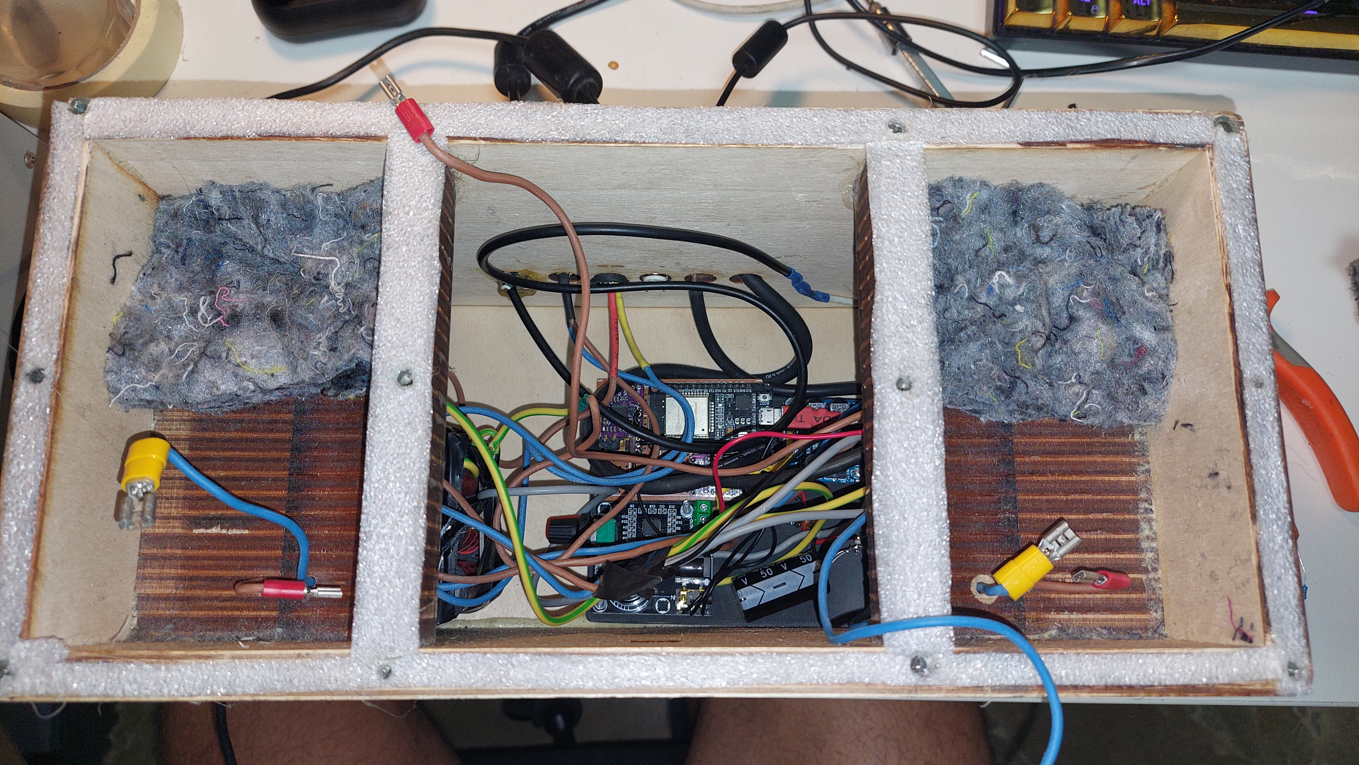
After the two parts of the enclosure were finished, the electronics were introduced. Then, before assembling them together, some textile damping material was placed inside the tweeter cavities to reduce standing waves and enhance the FR of these drivers.

The holes in the enclosure were used to add a USB programming port, a charging port, a power switch, a button and two jack outputs connected to the DAC circuits for development and measuring purposes.

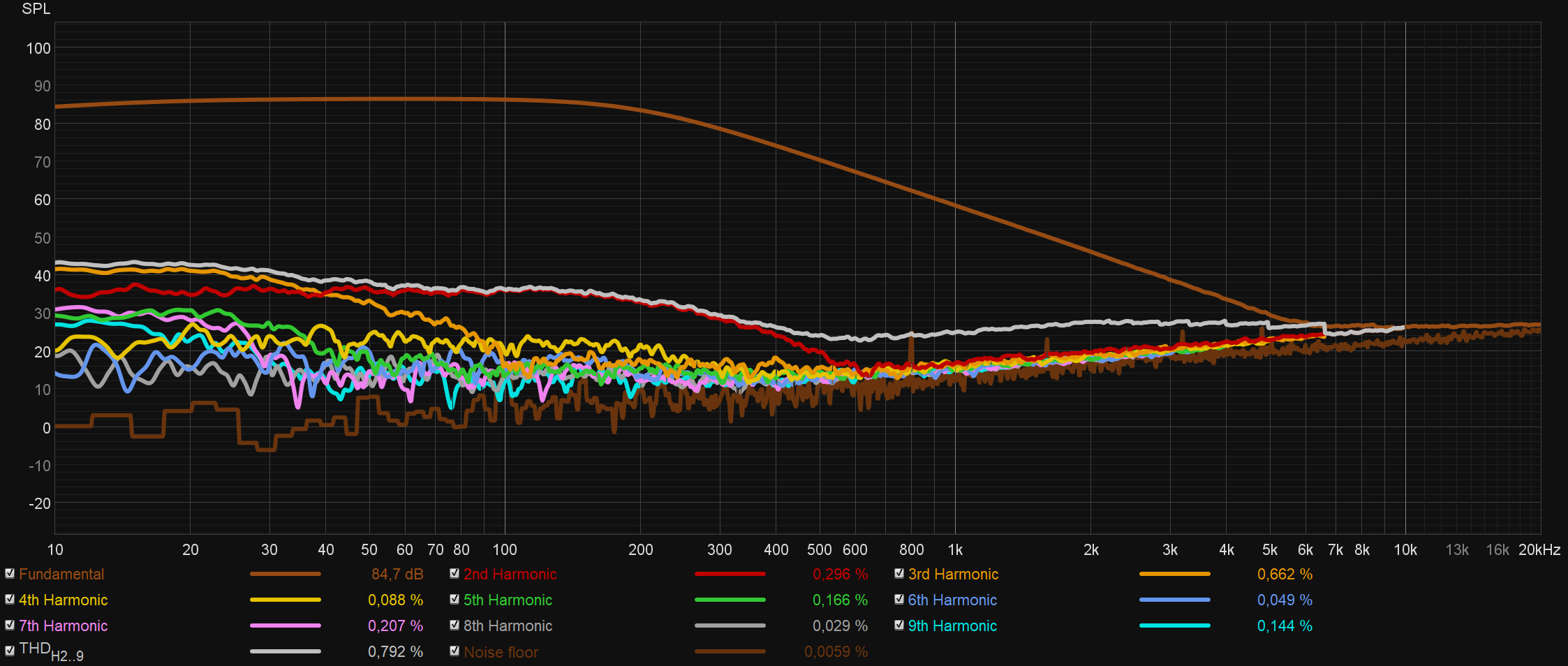
Filter adjustement and frequency response correction

After the system is built, the final task consists on correcting the acoustic FR. The first adjustment consists in the input gain adjustment of the amplifiers. For that purpose, various measurements were taken in a process of trial and error. The final adjustment included the introduction of a voltage divider with resistors to reduce the amplitude before the woofer amplifier. The tweeter amplifier was regulated by using the in-built variable resistor.

Raw frequency response measurement

The decisions on the bass frequencies must be taken by looking at the full system response, because the woofer channel sums the stereo signal into mono.

On the other hand, for high frequency correction, measurements need to be taken in mono to avoid interference between the two tweeters.

The measurements were made in an acoustically treated room that follows the LEDE (live-end dead-end) scheme.

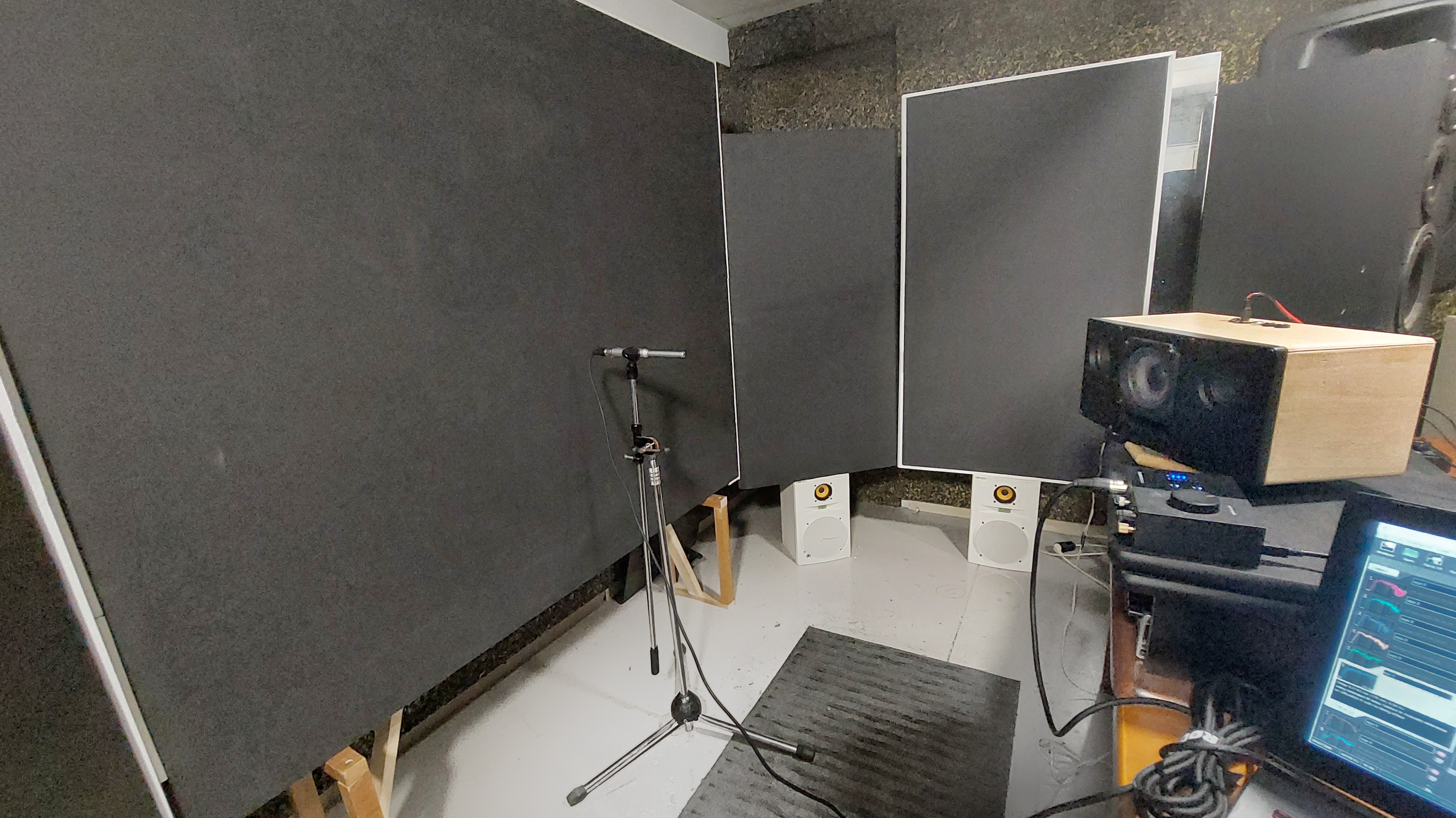
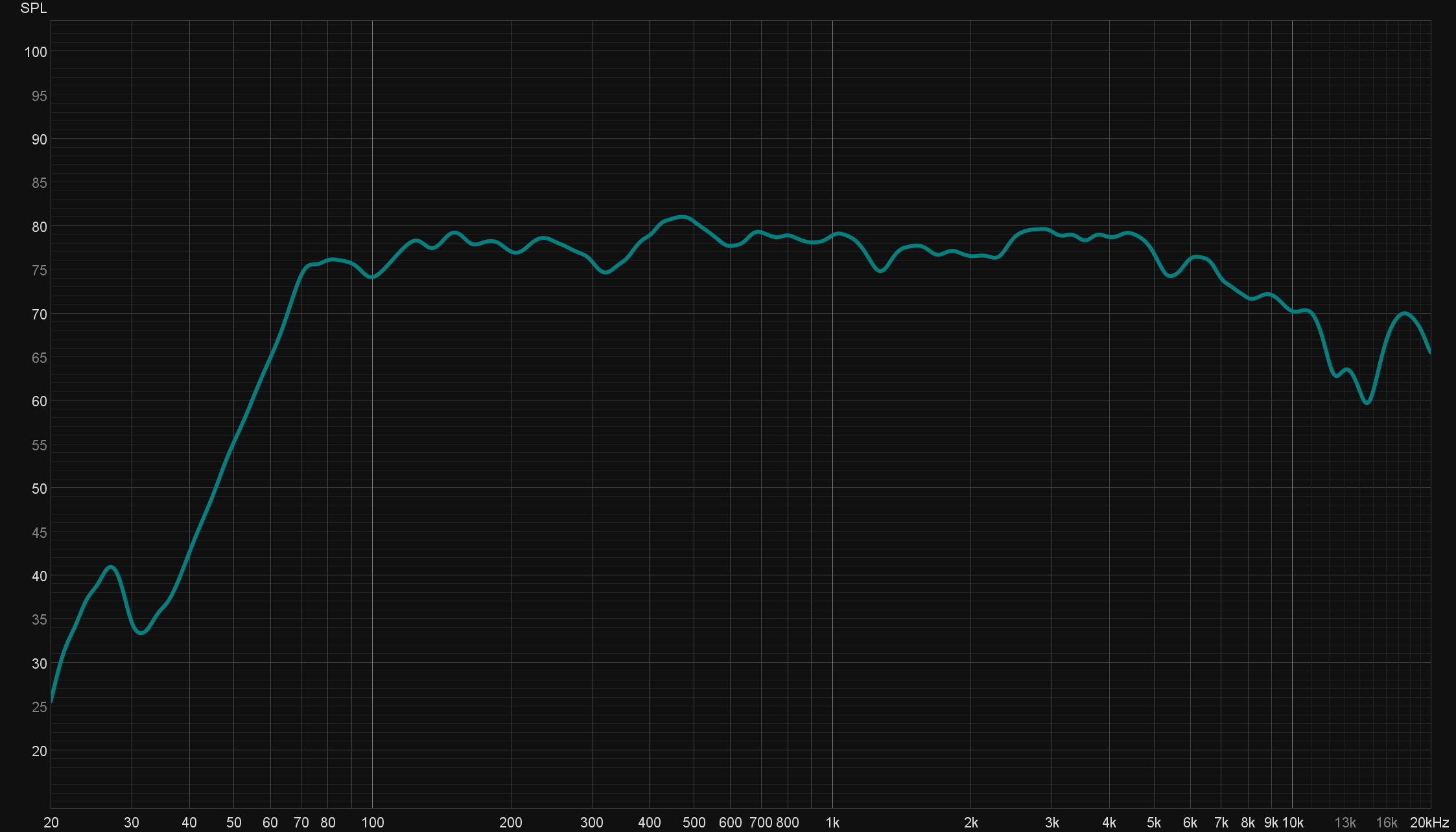
Full system measure

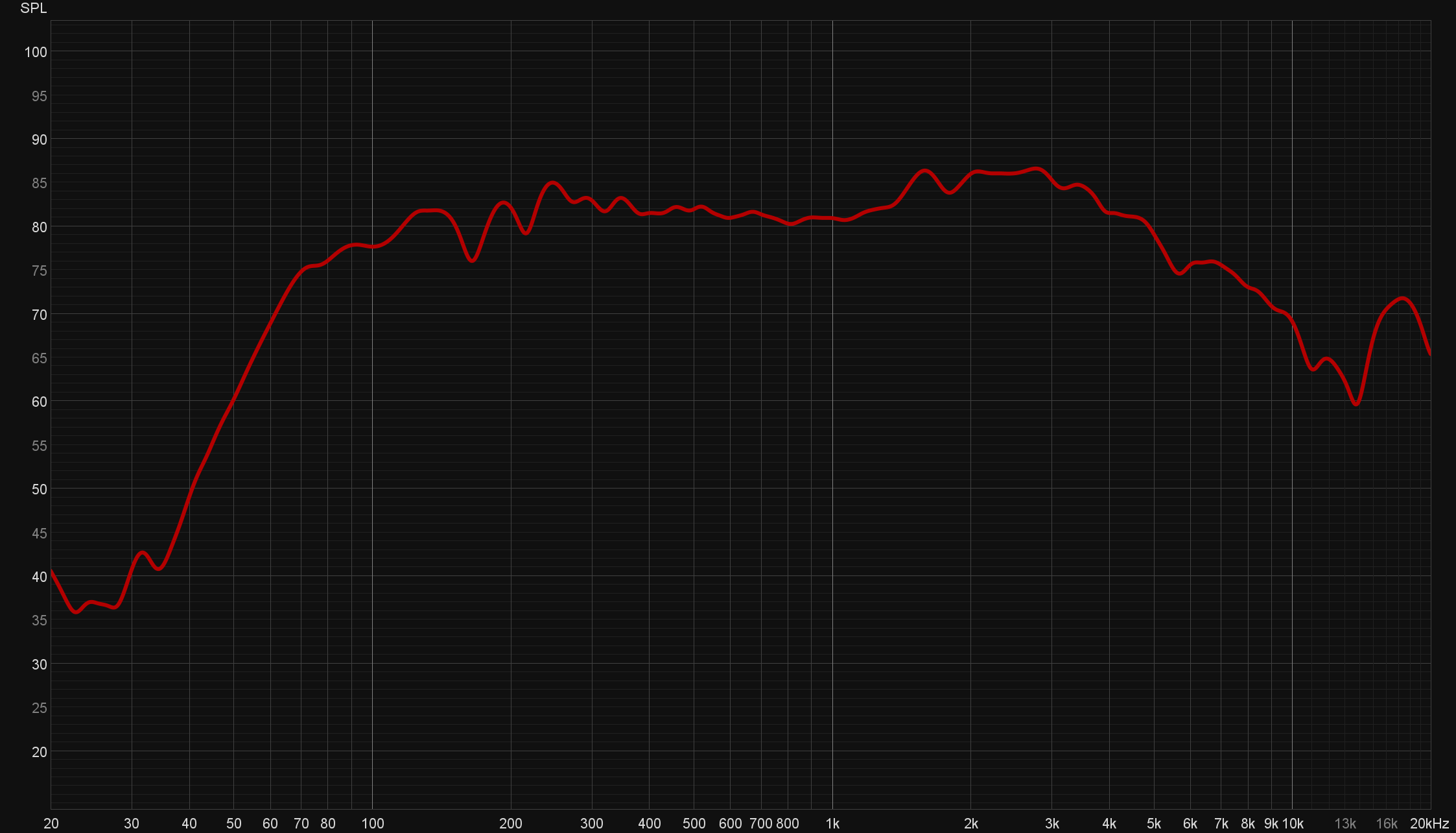
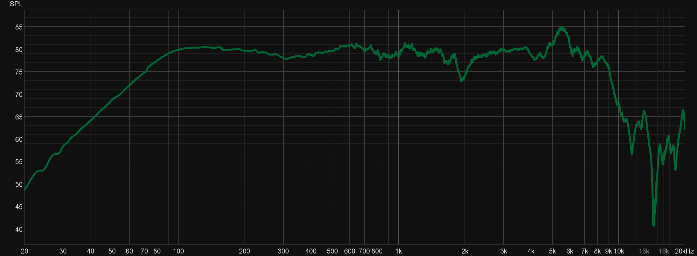
By looking at the graph, it is clear that the bass region needs to be boosted to match the higher frequency magnitude.

Apart from that, the crossover frequency is right, as there is not a significant dip or peak in it.

Left tweeter muted

Right tweeter muted

On the other hand, the FR of the two tweeters has a notorious build up around 2.5 KHz. Therefore, it will be needed to reduce the magnitude on this region.

DSP magnitude alignment

Bass correction

A bell filter was applied at 78Hz to increase the magnitude in the bass region.

$$\frac{s^2+125s+490^2}{s^2+50s+490^2}$$

The TF was discretized using the tustin method, giving the next discrete system.

$$\frac{1.001 z^2 - 1.999 z + 0.998}{z^2 - 1.999 z + 0.9989}$$

The code implementation is as follows.

Bass correction at 78Hz in dsp.h

 1
 2
 3
 4
 5
 6
 7
 8
 9
10
11
12
13
14
15
16
17

static float wyb = 0;
static float wyb_1 = 0;
static float wyb_2 = 0;
static float wub_1 = 0;
static float wub_2 = 0;

// 78Hz Bass Boost
static float Wf_78Hz_Boost(float wub)
{
	wyb = 1.998743507439808* (wyb_1 - wub_1) + 0.998017058334367 * wub_2 - 0.998866890476781 * wyb_2 + 1.000849832142414 * wub;

	wub_2 = wub_1;
	wub_1= wub;
	wyb_2 = wyb_1;
	wyb_1 = wyb;
	return wyb;
}

Treble reduction at 2KHz

To reduce the magnitude at 2KHz, the tweeter channel was processed with a bell filter that has a gain of 0,4.

$$\frac{s^2+8000s+14250^2}{s^2+20000s+14250^2}$$

The resulting TF is as follows.

$$\frac{0.8914 z^2 - 1.555 z + 0.7466}{z^2 - 1.555 z + 0.638 }$$

And finally, the implementation in the code.

 1
 2
 3
 4
 5
 6
 7
 8
 9
10
11
12
13
14
15
16
17
18
19
20
21
22
23
24
25
26
27
28
29
30
31
32
33
34
35

//Variables for 2KHz cut left
static float lyc = 0;
static float lyc_1 = 0;
static float lyc_2 = 0;
static float luc_1 = 0;
static float luc_2 = 0;

//Variables for 2KHz cut right
static float ryc = 0;
static float ryc_1 = 0;
static float ryc_2 = 0;
static float ruc_1 = 0;
static float ruc_2 = 0;

static float Wf_2kHz_Cut_L(float luc)
{
	lyc = 1.554677273766128 * (lyc_1 - luc_1) + 0.746611599629706 * luc_2 - 0.638016570899580 * lyc_2 + 0.891404971269874 * luc;

	luc_2 = luc_1;
	luc_1= luc;
	lyc_2 = lyc_1;
	lyc_1 = lyc;
	return lyc;
}

static float Wf_2kHz_Cut_R(float ruc)
{
	ryc = 1.554677273766128 * (ryc_1 - ruc_1) + 0.746611599629706 * ruc_2 - 0.638016570899580 * ryc_2 + 0.891404971269874 * ruc;

	ruc_2 = ruc_1;
	ruc_1= ruc;
	ryc_2 = ryc_1;
	ryc_1 = ryc;
	return ryc;
}

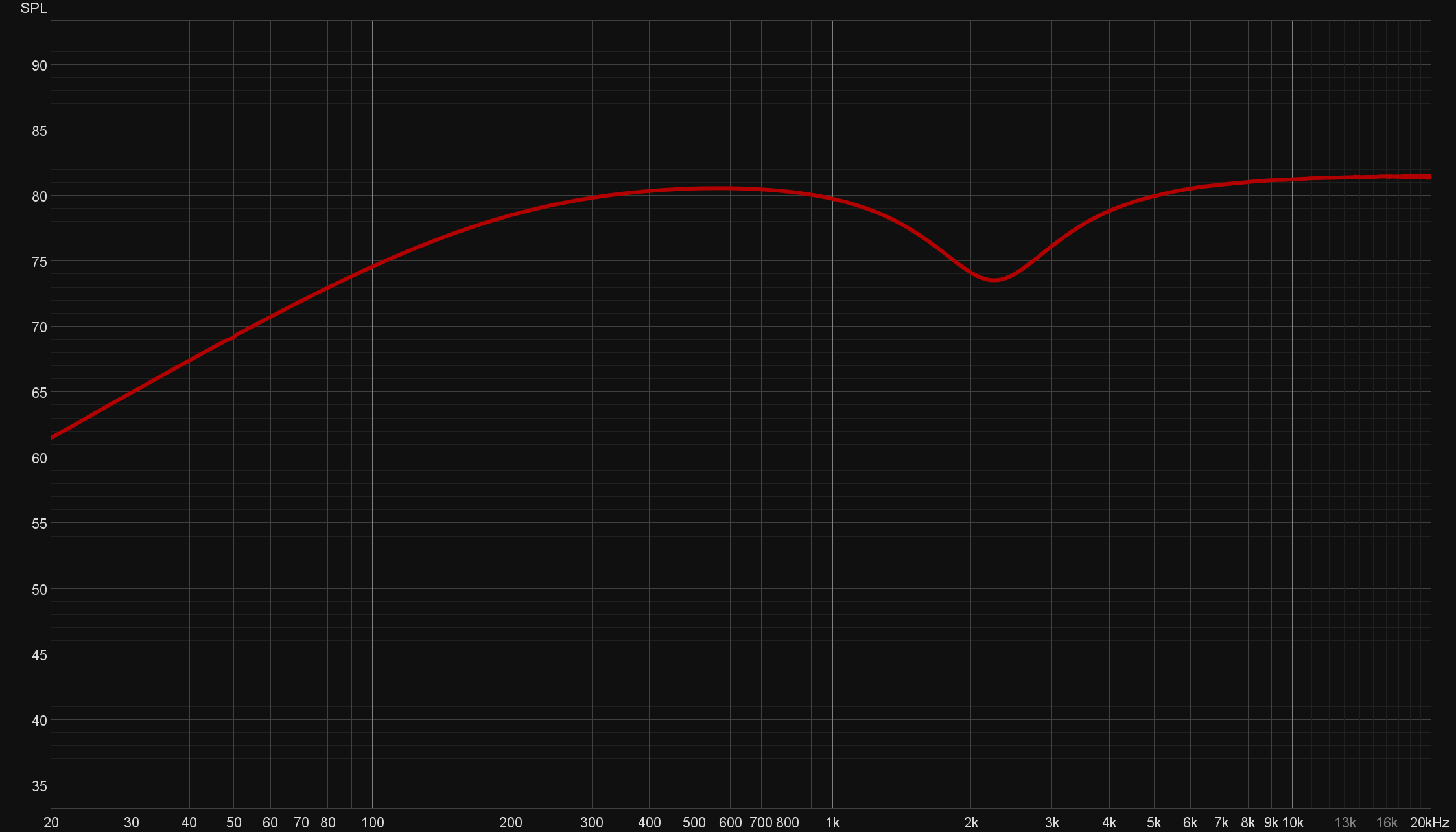
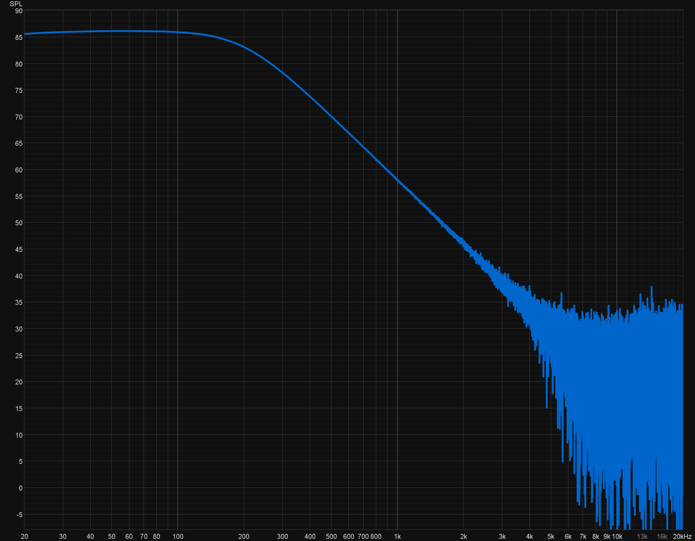
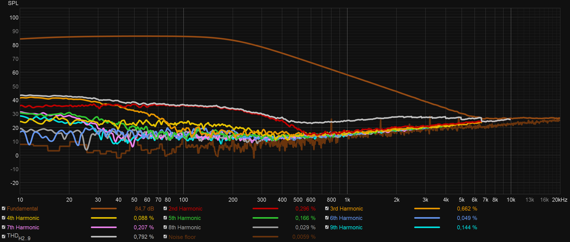
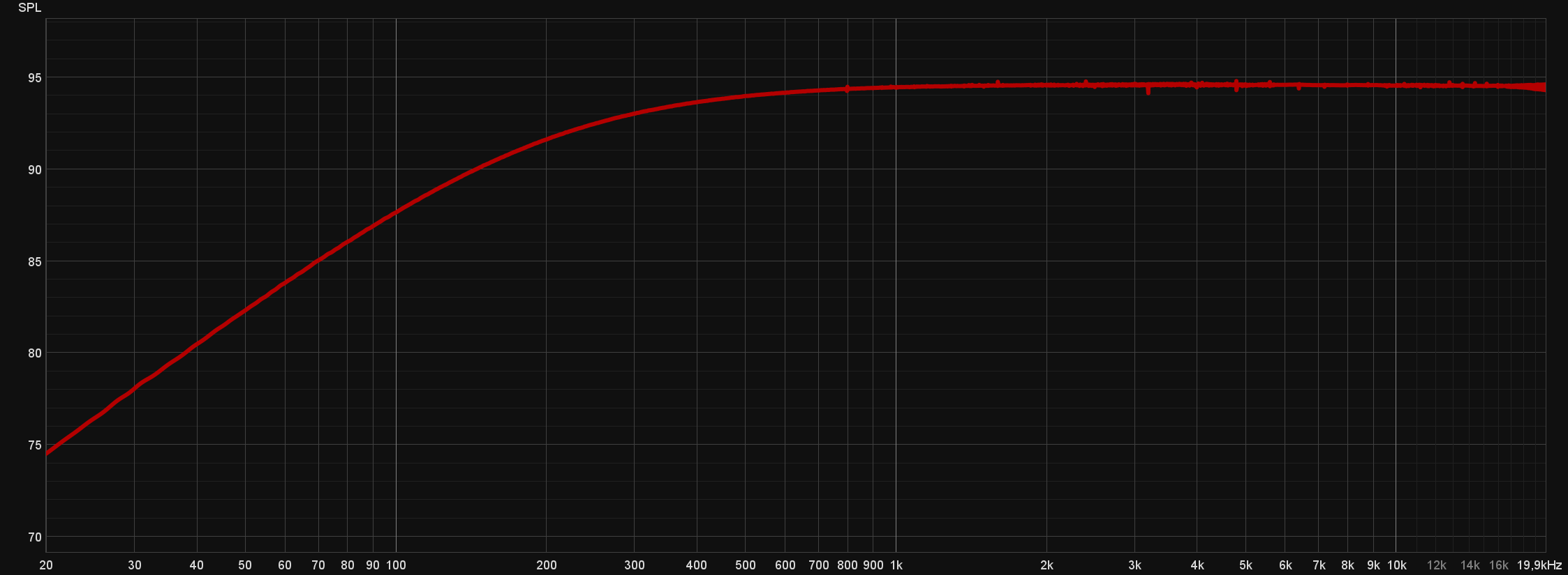
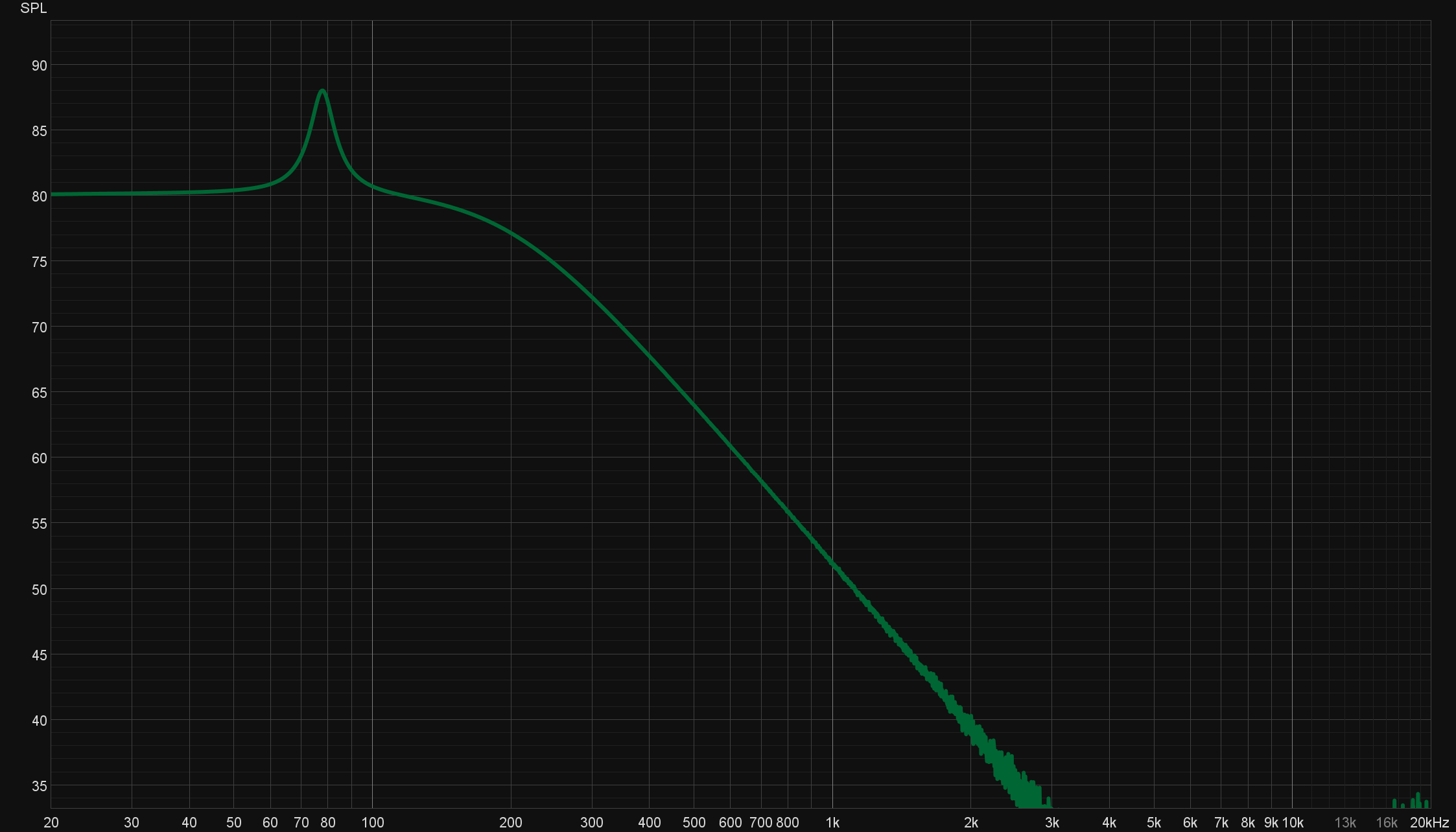
Corrected frequency response

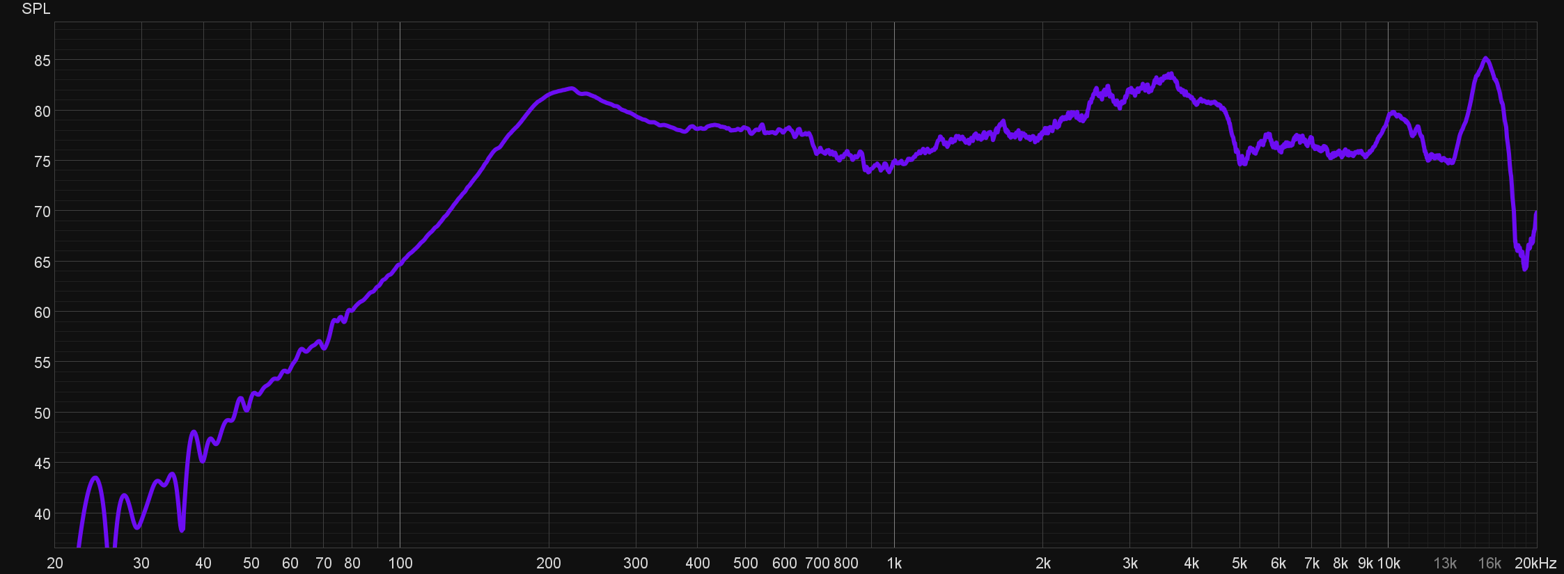
The next graph represent the FR of the full system in standard conditions.

As the graph shows, the FR improved enormously, and this is something that can be appreciated in the final sound without a doubt.

Note that the higher frequencies fall over 5KHz, due to the fact that is a stereo measurement in the center of the speaker where there exists a destructive interference. To evaluate the treble region, it is needed to do another measurement using only one channel and setting the microphone next to the tweeter.

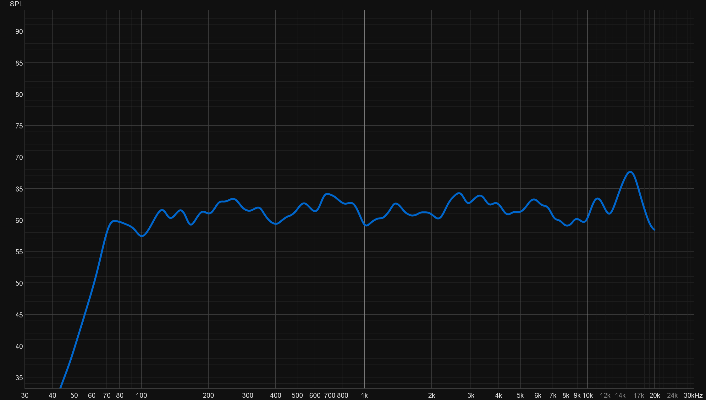
The next graph represents the FR of the right channel of the speaker. The measurement was done in the same conditions than the previous one.

Optimizing DSP operations

In this project, all of the signal processing has been done with floating point operations. This method has a much greater computational cost than designing the algorithms with bit-level operators.

Because the ESP32's FPU is not very powerful, as the number of filters increased, eventually, the processor couldn’t handle such amount of floating point operations, and there were missing samples that ruined the output signal.

As increasing the buffer size didn’t make a difference anymore, it was necessary to do some optimizations.

Discretization method

When testing the differences between Tustin and ZOH, there were cases in which the amount of floating point operations was different from one to the other. Knowing that the discretization method doesn’t make any noticeable difference in sound, it was decided to use the one which was computationally lighter in every case.

Optimizing maths

Apart from that, one thing that helped significantly is to reduce the floating point multiplications by using the distribuitive property. There are some coefficients that are multiplied by the same factor and then, are added in the difference equation.

High-Pass tustin filter, unoptimized vs optimized in dsp.h

 1
 2
 3
 4
 5
 6
 7
 8
 9
10
11
12
13
14
15
16

static float hpf_200Hz_L_Tustin(float u) //UNOPTIMIZED FILTER
{
	ly = 0.986025712688653 * u - 0.986025712688653 * lu_1 + 0.972051425377306 * ly_1;
	ly_1 = ly;
	lu_1 = u;
	return ly;
}


static float hpf_200Hz_L_Tustin(float u) //OPTIMIZED FOR CALCULATION ECONOMY
{
	ly = 0.986025712688653 * (u - lu_1) + 0.972051425377306 * ly_1;
	ly_1 = ly;
	lu_1 = u;
	return ly;
}

Results and conclusions

Power Specifications

The power handling of the speaker was measured as the maximum consumption power playing pink noise at maximum volume without clipping. As the power draw has short transients in time, a set of capacitors was used to maintain it as constant as possible.

The measured power was 18.7 W

Sound quality

The combination of stereo sound and a flat response over all the frequency spectrum provides a remarkable sound that fully satisfies the initial expectations. The data exposed in the measurements reflects the results of the project in terms of sound quality as it was explained at the beginning of the document.

Batery life

The battery life was tested in the conditions that are expected to be the regular use of the final customer. That means, constant music playback at around 60% max volume.

The implementation of DSP in a µC that lacks of dedicated hardware for such purpose resulted in a high power consumption when the speaker was in idle state. To be exact, the µC and the buck converter alone drain 3.3W constantly.

Even with that, the battery lasted for more than 5h in all the tests. The best case scenario reported more than 8h, and the worst was around 5h, when the music was played at full volume the entire test.

Conclusions

Among all the difficulties related to the development process, the final product meets the initial objectives in all aspects.

Apart from that, it’s worth to mention that the means to carry out acoustic quality measurements were good but not optimal. Even though the room was acoustically treated, some of the irregularities seen in the acoustic FR are caused by the room modes itself.

To prevent that, the measurements should have been done in an anechoic chamber capable of absorbing most of the reflections that cause nulls and peaks in the measured FR.

ESP32

Bibliography

[1] Vance Dickason.The Loudspeaker Design Cookbook. Google-Books-ID: _K3SAAAACAAJ. Audio Amateur Press, Dec. 2007. 275 pp.isbn: 978-1-882580-47-7 (cit. on pp. 23, 27).

[2] Thiele/Small parameters. In:Wikipedia. Page Version ID: 1100463633. July 26, 2022 (cit. on p. 24).

[3] Knud Thorborg and Claus Futtrup. “Electrodynamic Transducer Model Incorporating Semi- Inductance and Means for Shorting AC Magnetization”. In:J. Audio Eng. Soc59.9 (2011), pp. 612–627 (cit. on p. 24).

[4] Morten H. Knudsen and J. Grue Jensen. “Low-Frequency Loudspeaker Models That In- clude Suspension Creep”. In:Journal of the Audio Engineering Society41.1 (Feb. 1, 1993). Publisher: Audio Engineering Society, pp. 3–18 (cit. on p. 24).

[5] Bluetooth A2DP API - ESP32 - — ESP-IDF Programming Guide latest documentation.url: https://docs.espressif.com/projects/esp-idf/en/latest/esp32/api-reference/ bluetooth/esp_a2dp.html(visited on 09/10/2022) (cit. on p. 34).

[6] Acoustics/Fundamentals of Psychoacoustics - Wikibooks, open books for an open world.url: https : / / en. wikibooks. org / wiki / Acoustics / Fundamentals _ of _ Psychoacoustics (visited on 09/11/2022) (cit. on p. 36).

[7] Ethan Winer.The Audio Expert: Everything You Need to Know About Audio. Google-Books- ID: 6FoPEAAAQBAJ. Routledge, Dec. 15, 2017. 809 pp.isbn: 978-1-351-84007-1 (cit. on p. 39).